EVOLUTIONARY SEARCH FOR MODELS OF
PLANARIAN REGENERATION USING
EXPERIMENTAL DATA

by
Marianna Viktorovna Budnikova

A thesis
submitted in partial ful llment
of the requirements for the degree of
Master of Science in Computer Science
Boise State University

December 2014

c 2014
Marianna Viktorovna Budnikova
ALL RIGHTS RESERVED

BOISE STATE UNIVERSITY GRADUATE COLLEGE

DEFENSE COMMITTEE AND FINAL READING APPROVALS

of the thesis submitted by

Marianna Viktorovna Budnikova

Thesis Title: Evolutionary Search for Models of Planarian Regeneration Using Experimental Data

Date of Final Oral Examination: 17 October 2014

The following individuals read and discussed the thesis submitted by student Marianna Viktorovna Budnikova, and they evaluated her presentation and response to questions during the final oral examination. They found that the student passed the final oral examination.

Timothy Andersen, Ph.D. Chair, Supervisory Committee
Jeffrey W. Habig, Ph.D. Member, Supervisory Committee
Elena A. Sherman, Ph.D. Member, Supervisory Committee

The final reading approval of the thesis was granted by Timothy Andersen, Ph.D., Chair of the Supervisory Committee. The thesis was approved for the Graduate College by John R. Pelton, Ph.D., Dean of the Graduate College.

Dedicated to my husband, Allen.

ACKNOWLEDGMENTS

Thank youto myhusband, Allen. You have given me love and support throughout my schooling and thesis writing. The walks on the Greenbelt and rest breaks you encouraged me to take between studying and work not only kept me sane, but allowed me to finish my thesis on time! Thank you to my parents for letting me pursue my dream of becoming a computer scientist so far away from home. Thank you to my host parents who became my second set of parents while I followed my software dream and fought code bugs.

Dr. Tim Andersen, thank you for introducing the wonders of artificial intelligence to me. Taking the second introductory computer science course from you during my undergraduate studies inspired me to pursue computing further. Thank you for all the inspirational conversations we had about genetic algorithms, bioinformatics, Disneyland, and life. You are a super-awesome adviser. I would like to thank past and present employees of Crowley Davis Research for their hard work on the Cellsim platform and for making it available for these studies. This work was made available through an NSF-CDI grant (EF-1124665).

ABSTRACT

The ability of science to produce experimental data greatly surpasses our cur rent ability to e ectively visualize, conceptualize, and integrate the vast volumes of available data into a uni ed understanding of how complex biological systems work. This inability is a hindrance to scienti c progress, and is particularly daunting when one considers multidimensional and shape-based observations as in the field of regenerative biology. For example, for at least the last 200 years, scientists have been interested in the exceptional ability of Planaria to regenerate lost tissues from damage, and there is a large amount of experimental data available on this organism.

However, until recently, none of these experiments had been collected into a single database. To this end, a repository (PlanformDB) has been created that includes formal descriptions of planaria experiments, including morphological descriptions of the worms using a graph formalism. PlanformDB opens the door to automated, formal approaches for analyzing and understanding the large amount of available experimental data for planaria.

This work seeks to automate the search for models of planaria regeneration against the Planform database with experiments. Regeneration models not only help the understanding of how planarians maintain their shape based on the experiments observed up to today, but also provide a tool to predict the outcomes of future experiments. An automated model discovery framework was setup to simulate the experiments described in PlanformDB using an agent-based modeling platform com bined with evolutionary search to identify plausible mechanisms for the biological behavior.

The automation has been achieved through the linking of the simulation platform to Plan form DB and development of fitness metrics that enable the evolutionary search. The proposed fitness metrics were developed, implemented, and then evaluated by assessing their tness landscapes. A fitness landscape represents the range of possible fitness values that can be assigned to various models. In this work, the roughness, a fitness, and the presence of local maxima in the fitness landscapes were evaluated for the proposed fitness functions. To further test the utility of the proposed fitness functions, a simple evolutionary search was performed.

ABSTRACT………………………………………..
LIST OF TABLES……………………………………
LIST OF FIGURES…………………………………..
LIST OF ABBREVIATIONS ……………………………

1 Introduction………………………………………

1.1 Problem Description. . . . . . . . . . . . . . . . . . . . . . . . . . . . . . . . . . . . . . . .
1.2 Thesis Statement . . . . . . . . . . . . . . . . . . . . . . . . . . . . . . . . . . . . . . . . . .
1.2.1 Objectives . . . . . . . . . . . . . . . . . . . . . . . . . . . . . . . . . . . . . . . . . .
1.2.2 Procedures . . . . . . . . . . . . . . . . . . . . . . . . . . . . . . . . . . . . . . . . .
1.3 Modeling a Classic Planaria Regeneration Experiment . . . . . . . . . . . . .
1.4 Tools. . . . . . . . . . . . . . . . . . . . . . . . . . . . . . . . . . . . . . . . . . . . . . . . . . . .
1.4.1 Computational Platform and Evolutionary Search . . . . . . . . . . .
1.4.2 A Database for Storing Planarian Experiments . . . . . . . . . . . . .
1.4.3 ASample Regeneration Model . . . . . . . . . . . . . . . . . . . . . . . . . .

2 Graph Edit Distance Fitness Function …………………..

2.1 The Graph Formalism for Comparing Worms . . . . . . . . . . . . . . . . . . . .
2.1.1 Design of a Connected Component Analysis Algorithm to Con
vert Cell Simulation Output into Graph Representations . . . . .
2.1.2 Graph Edit Distance as a Fitness Function. . . . . . . . . . . . . . . . .
3 Overlay Fitness Function …………………………….
3.1 Comparing Two Morphologies by Overlaying a Graph with a Blob of Cells . . . . . . . . . . . . . . . . . . . . . . . . . . . . . . . . . . . . . . . . . . . . . . . . . . . .
3.2 Graph-to-Line Conversion . . . . . . . . . . . . . . . . . . . . . . . . . . . . . . . . . . .
4 Dierence Distributions Fitness Function…………………
4.1 Comparing Two Morphologies by Calculating Dierence Distributions of Their Resources . . . . . . . . . . . . . . . . . . . . . . . . . . . . . . . . . . . . . . . . .
5 Experiment Database Reader and Writer…………………
5.1 Experiment Database Reader of Morphologies and Experiments . . . . . .
5.2 Experiment Database Writer of Morphologies . . . . . . . . . . . . . . . . . . . .
6 Automated Experiment Extraction and Application…………

7 Results………………………………………….
7.1 Evaluation of the Cellular Snapshot-to-Graph Conversion Algorithm . .
7.1.1 Cell Connectivity Distance Threshold Effects on Region Determination . . . . . . . . . . . . . . . . . . . . . . . . . . . . . . . . . . . . . . . . . . .
7.2 Evaluation of the Proposed Fitness Functions . . . . . . . . . . . . . . . . . . . .
7.2.1 Dierence Distributions Fitness Function Evaluation. . . . . . . . .
8 Conclusions ………………………………………
8.1 Automation of Search for Regeneration Models . . . . . . . . . . . . . . . . . . .
8.2 Future Work. . . . . . . . . . . . . . . . . . . . . . . . . . . . . . . . . . . . . . . . . . . . . .
8.2.1 Organs . . . . . . . . . . . . . . . . . . . . . . . . . . . . . . . . . . . . . . . . . . . .
8.2.2 Combination of Fitness Functions. . . . . . . . . . . . . . . . . . . . . . . .
8.2.3 Cellular Morphologies Beyond One Layer . . . . . . . . . . . . . . . . . .

REFERENCES………………………………………

LIST OF TABLES

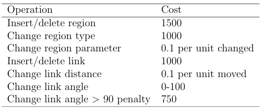
2.1 This table presents the graph edit costs used for graph edit distance calculations in this manuscript. . . . . . . . . . . . . . . . . . . . . . . . . . . . . . . .
2.2 Evaluation of conversion equations to generate tness values from graph edit distance values. The rst row presents the data for the graph of the target individual. The first and second columns of the table show the ID and the image of the morphology graph. The third column presents the graph edit distance value obtained from comparison of the graph against the target graph using graph edit distance algorithm. The fourth through the ninth column show the fitness value produced by plugging in the constant in the column header into Equation 2.1. . . . . .
7.1 Single cut morphology experiment results for simulation snapshot to graph conversion and graph edit distance comparison . . . . . . . . . . . . . .
7.2 Threshold value in influence on snapshot to graph conversion algorithm . .
7.3 Comparison of fitness function landscapes to the ideal fitness function landscape. . . . . . . . . . . . . . . . . . . . . . . . . . . . . . . . . . . . . . . . . . . . . . . . .

7.4 Statistics obtained from analyzing the atness of the fitness landscapes. The first column shows the name of the landscape analyzed. Di Dist refers to the di erence distributions evaluator and Graph to the graph edit distance evaluator. The second column presents the total number of at surfaces in the landscape, the third column shows the percentage of the total landscape occupied by the biggest at surface, and the last column shows the percentage of the landscape occupied by the at surfaces. . . . . . . . . . . . . . . . . . . . . . . . . . . . . . . . . . . . . . . . . . . . . . . . . .

7.5 Statistics obtained from analyzing the roughness of the fitness land scapes. The first column shows the name of the fitness landscape, and the second column shows the number of local maxima in the landscape.
7.6 The runtime of di erence distribution histogram creator implementations in C and Python for morphology in column one are shown in columns two and three, respectively. The speedup provided by the C implementation of the histogram creator is shown in column four. The last row of the table shows the average runtimes.. . . . . . . . . . . . . . . . . .
7.7 Difference distributions for morphologies with different gene knockouts performed. The first row in the table presents the difference distribution data for the target morphology. . . . . . . . . . . . . . . . . . . . . . . . . . . .

LIST OF FIGURES

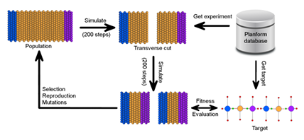
1.1 This gure depicts a classic planaria regeneration experiment involving a transverse cut of an intact worm, followed by the regeneration products for each fragment. The real experiment is shown in (a) along with the (b) simulation and (c) graph representations. In each case, the second panel represents the worms immediately following the cut, whereas the third panel depicts the regeneration outcome at a later time. 11 1.2 CSGA evolutionary search ow. . . . . . . . . . . . . . . . . . . . . . . . . . . . . . . .

1.3 Awild-type planarian organism (a), along with its graph representation (b) in the Planform software tool. . . . . . . . . . . . . . . . . . . . . . . . . . . . . .

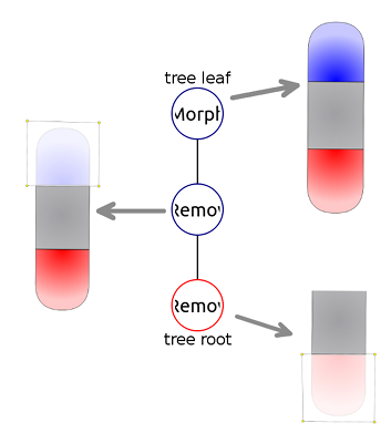
1.4 A manipulation tree for an experiment involving removal of the head and tail regions. . . . . . . . . . . . . . . . . . . . . . . . . . . . . . . . . . . . . . . . . . . .

2.1 The assignment of a cell to a state depends on the molecular concentrations of cell-state indicators. The di erentiate state of cells are color-coded to enable visual distinction of cells and the composition of a region: head (blue), trunk (yellow), and tail (purple). Within a given cell, the location of a given resource can be distributed between the internal compartment (e.g., cytosol) and the surface (e.g., membrane). Concentrations of representative resources inside (I) and on the surface (S) are provided. In this example, both Cell 1 and Cell 2 are assigned to a trunk state and Cell 3 is assigned to a trunk state, since the concentrations of the indicator molecules (iCell and tCell, respectively) for these states are the highest. . . . . . . . . . . . . . . . . . . . . . . . . . . . . . . .

2.2 Pseudocode for connected component analysis recursive algorithm to separate a list of cells taken from the simulation snapshots into discrete morphology regions. . . . . . . . . . . . . . . . . . . . . . . . . . . . . . . . . . . . . . . . .

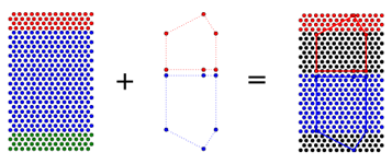
3.1 In this example of overlaying a cellular morphology with a graph morphology, the cellular morphology consists of three regions, head (red), trunk (blue), and tail (green), while the overlayed graph only has a head and atrunk. Whenthegraph is overlayed with the cellular morphology, some of the cells do not match the type of the overlayed graph (colored in black). . . . . . . . . . . . . . . . . . . . . . . . . . . . . . . . . . . . . . . . . . . . . . . . .

3.2 Overlay difference fitness evaluator. . . . . . . . . . . . . . . . . . . . . . . . . . . . .

3.3 Sample conversion of a two-node morphology graph into lines. Three point types calculated during the conversion algorithm are indicated. . .

4.1 Distribution calculation using using a cell processor . . . . . . . . . . . . . . .
4.2 Fitness calculation using difference distributions . . . . . . . . . . . . . . . . . .
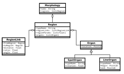
5.1 UML diagram for the Plan form database morphology. . . . . . . . . . . . . .
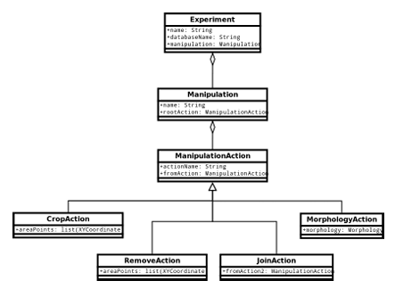
5.2 UML diagram for the Plan form database experiment. . . . . . . . . . . . . .
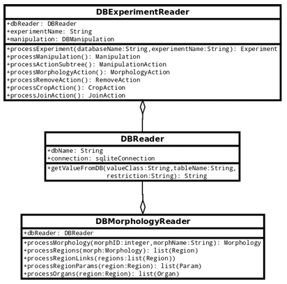
5.3 UML diagram for the Plan form database reader. . . . . . . . . . . . . . . . . . .
5.4 UML diagram for the Plan form database writer. . . . . . . . . . . . . . . . . .
5.5 Sample SQLite queries to call to Plan form DB.. . . . . . . . . . . . . . . . . . . .
5.6 Sample calls of Python database writer functions. . . . . . . . . . . . . . . . . .
6.1 The graphical user interface for the Cell Sim simulation platform. . . . . .
6.2 Example of applying a PlanformDB experiment manipulation (injection of Lysis) to a cellular model in CellSim. . . . . . . . . . . . . . . . . . . . . .
6.3 UML diagram for the PlanformDB experiment manipulation applica tor. . . . . . . . . . . . . . . . . . . . . . . . . . . . . . . . . . . . . . . . . . . . . . . . . . . . .
6.4 Pseudocode for extraction of points falling inside the manipulation polygon formed by action points . . . . . . . . . . . . . . . . . . . . . . . . . . . . . .
7.1 Fitness function evaluation on polar model with two gene regulatory regions removed independently and gradually returned. The x-axis shows the effect value of the knocked out regulatory region. The y-axis presents the fitness value assigned to the simulated model with a given promoter effect. The graph edit distance function fitness is shown in yellow, overlay in blue, and difference distributions in red. . . . . . . . . . .

7.2 A cellular morphology generated in CellSim using a model with small head and tail regulatory region e ects as well as its graph representation.

7.3 Fitness function evaluation of the polar model with hCell and tCell promoters knocked out and gradually returned. . . . . . . . . . . . . . . . . . . .

7.4 Fitness function evaluation of the polar model with low hCell and tCell decay rates in which hCell and tCell regulatory regions were knocked out and gradually returned. . . . . . . . . . . . . . . . . . . . . . . . . . . . . . . . . . .

7.5 A time series graph for an evolutionary search for a target capable of producing stable head and tail regions. . . . . . . . . . . . . . . . . . . . . . . . . .

LIST OF ABBREVIATIONS

API

Application Programming Interface

CellSim

Cellular Simulation platform

CSGA

CellSim Genetic Algorithm

GA

Genetic Algorithm

GUI

Graphical User Interface

PlanformDB

Planform database

Subunit-

A part of an abstracted cell in CellSim that facilitates cell growth and division

CHAPTER 1

INTRODUCTION

1.1 Problem Description

Robust regulatory control of organism morphology, including tissue and organ regeneration, appears in many di erent animal and plant kingdoms and species, and has been extensively studied and analyzed by scientists [7, 21, 22]. Despite extensive e ort and focus on this core problem in biology, and bringing to bear the incredibly powerful modern analytic tools developed by molecular biologists and bioninformaticians, the problem of deriving, understanding, and learning to control the robust, large-scale patterning properties of complex systems from the data about its components is yet to be solved.

Take, for example, planaria worms. Planaria are free-living atworms that exhibit much of the complexity of the vertebrae systems: a well-defined nervous system with most of the same neurotransmitters as human brains, eyes, intestinal tract, and bilateral symmetry [2]. Planaria have the sensory capabilities to detect light [11, 10], chemical gradients [30, 28], vibration [14], electric elds [11], magnetic fields [13, 8], and weak radiation [9]. Yet even though the main components constituting the planarian morphologies are known and have been described extensively, the features guiding the regulatory and patterning properties of planarians remain largely unknown.

An especially interesting feature of planaria worms that has been puzzling the minds of scientists for over 200 hundred years is the atworms ability to recover from even severe injuries. In 1776, Peter Simon Pallas discovered that bisecting a planarian organism did not kill it [35]. Instead, the two pieces of the cut worm regenerated into two intact worms (Fig. 1.1a). In 1898, Thomas Morgan showed that a cut worm piece constituting 1/279th of the total worm weight was able to regenerate into a new worm with many internal organs and a bilateral symmetry
[31]. Since Pallas and Morgans discoveries, many more experiments have been performed on planaria aiming to understand the mechanics behind the animals remarkable regenerative capabilities [33], [23].

However, scientists still lack a complete understanding of the planarian regeneration process [23]. In an attempt to explain the processes guiding the atworm regeneration, several models of planarian regeneration have been proposed. Among these models are the gradient model [29], serial threshold theory of regeneration [38], reaction diffusion mechanisms of patterning [39, 15], bioelectric- electrophoretic model [19], dorsoventral interaction model [17], and the intercalary regeneration model [1]. However, not a single proposed model explains comprehensively the mechanisms of all the known components of planarian regeneration, and it is likely that the worm utilizes a complex combination of several of these strategies, and perhaps even strategies that have yet to be elucidated, to achieve its robust regenerative ability. Unfortunately, it is extremely di cult to develop a model by hand that can accurately explain the hundreds of experiments performed on planaria worms currently found in the literature. Even if such a model existed, with new experiments and findings being continually published, the model is likely to need continued parameter adjustment and fine tuning in order to explain these experiments. The problem of finding a regeneration model to t all the experiments performed on planarians can be made
more tractable by using computational tools to assist researchers in model formation, fine tuning, and testing.

Agood example of such a tool is an evolutionary search algorithm combined with a cell-based modeling platform (CellSim Genetic Algorithm, or CSGA) used by the Andersen lab to discover and tune models of planarian regeneration [3]. Evolutionary search algorithms are inspired by biological evolution and based on the principle of survival of the ttest. Often regarded as generate-and-test algorithms, evolutionary algorithms use operators like mutation and crossover on populations of individuals to generate previously unseen individuals and test the goodness of these individuals via fitness evaluation [37]. An automated evolutionary algorithm can be used to combine and adjust the currently existing regeneration models to find a model that would be able to explain all the planarian regeneration experiments.

A big issue in automatized model discovery is evaluation of regeneration models against experiments found in the literature. Most regeneration models describe the metabolic states of the worm, which are di cult to evaluate due to the temporal variations in the worms metabolic states. Shape is a more objective way of assessing and validating metabolic state of an organism. When de ned using a standardized, controlled vocabulary, shape allows organisms to be described in an unambiguous fashion. Shape-based ontologies have been successfully applied to describing organisms and separate organs in the elds of biology and medicine. For example, the EQ method used entities (e.g., head, eye, tail) and associated qualities (e.g., small, round, reduced length) to describe the phenotypes of mice [6]. The Edinburgh Mouse Atlas Project (EMAP) implemented a spatio-temporal framework for capturing spatially organized and mapped data, in which a directed acyclic graph (DAG) was used to represent is-a-part-of relationships between tissues and organs of a mouse embryo [5]. Maglia et al. described a generic anatomical ontology that can be applied to different amphibian species, where the anatomy of an organism is described as a semantic network consisting of concepts and relationships, such as is-fused-to, is-formed-from [27]. The utility of shape ontologies goes beyond the descriptions of species phenotypes: shape formalisms have been applied in clinical diagnostics and analysis of tumor growth [36].

One of the main reasons for the popularity of shape-based ontologies is exibility. Shapes of organisms or organs described using a standardized language can be easily juxtaposed using computational methods. The computational exibility of shape-based ontologies works in favor of automatizing the search for planarian
regeneration models. Recently, the Levin lab at Tufts University developed a shape based formalism for describing planarian morphologies as graphs of connected regions [26]. Flexible graph notation allows the organisms to be described in terms of nodes connected by links at speci c angles. This formalism led to the implementation of a database for storing planarian morphologies and the experiments performed on planarians reported in the literature (PlanformDB) [25]. The database stores the experiment manipulations as a tree with planarian morphologies as leaves, which allows representation of a variety of experiments that can be performed on planaria. The Levin lab is working on populating this database (PlanformDB) with all experiments performed on planaria currently found in literature.

The introduction of the database of experimental manipulations and outcomes will revolutionize the process of creating and validating models of planarian regeneration. Using PlanformDB, scientists will be able to search for morphologies that match the shape of the proposed regeneration model. While the majority of databases allow the experiments to be searched by keywords, the PlanformDB database enables searching experiments with the worms shape as the key. Graph comparison algorithms allow discovery not only of exact morphology matches but also ones that are similar to the sought-for shape. Graph-matching algorithms can be used to automate the validation of proposed regeneration models against the regeneration experiments found in literature. In addition to validation of regeneration models, the integration of PlanformDB can help create new models of regeneration if combined with an automatic tool to tweak the regeneration model parameters. CSGA perfectly ts the
description of such a tool. I have integrated the database of experiments and their outcomes (PlanformDB) into the CSGA evolutionary search engine with the aim of developing an automated system for searching and validating computational models of development. In this system, an experiment can be pulled from the database and simulated in the simulation platform. In the past, in order to specify an experiment to be run in the cell-based platform, the user had to manually create a sheet of cells and specify operations to be performed on the morphology, such as cuts and injection of lysis or RNAi. This process of creating an experiment setup was painfully ine cient and slowed down the search for computational models of the planarian regeneration. The new automated system includes automatic access to the database for searching and pulling the experiments and morphological outcomes to use during the evolutionary search.

Models found by the evolutionary search can be evaluated against the planarian experiments in PlanformDB. However, to evaluate models against experiments during the evolutionary search, exible tness functions are needed. As a part of this work, I developed a tness function in which cellular outcome for a model generated by the simulation platform is converted into the graph representation and compared against the target individual from PlanformDB using the graph edit distance metric [12, 26]. The graph edit distance evaluator is a very exible tness function, since the graph formalism can be used in simulation platforms other than CellSim. However, a weakness of the graph edit distance evaluator is that it does not directly provide molecular targets for individual cells, but rather operates at the abstract level of a planarian morphology.

As a regeneration model is evaluated, it is benefecial to consider several features of the simulation outcome, including the general shape of the worm and its metabolic state. Fitness functions that evaluate an individual based on several features during the evolutionary search are called multi-objective fitness functions and are used to expand the evolutionary fitness landscape, as well as provide multiple search directions for the evolutionary algorithm [20]. During the run of the evolutionary search, a set of individuals resembling the target may be found. These individuals may differ slightly by the sizes of their regions or by the constants in their metabolic networks, but they all equally can be attributed as solutions. Using multiple fitness functions to expand the evolutionary search will expand the set of acceptable individuals and thus greatly speed up the search for regeneration models. Considering some of the features may be in con ict with each other, by expanding the set of acceptable solutions, the evolutionary search may find solutions that would be impossible to discover by using a fitness function based only on one metric [18]. From these considerations, several additional fitness functions were developed to evaluate the models of regeneration, in addition to the already proposed graph edit distance fitness function. In this work, three fitness evaluators are described and evaluated: the previously mentioned graph edit distance evaluator, and the overlay and difference distributions fitness functions. Each fitness function is evaluated by formally analyzing the roughness and fatness of the fitness landscapes produced by the evaluators. The utility of the fitness functions is also addressed by performing a simple evolutionary search for a target model capable of regenerating head and tail regions after a transverse cut is performed on the individual.

1.2 Thesis Statement

1.2.1 Objectives

The aim of this thesis is to automate the evolutionary search and discovery of com putational models of planaria regeneration that faithfully reproduce experimental outcomes reported in the literature. Automation of the evolutionary search required development of flexible fitness metrics and integration with a database of existing experiments and experiment outcomes. This thesis ful fills the following objectives:

1. To develop robust techniques for comparing cellular models from the simulation platform to the search targets taken from the experiment database.
2. Toautomate the extraction of experiment manipulations and morphologies from the experiment database to the cellular platform.
3. To automate application of experiment manipulations from the experiment database to the cellular morphologies.

1.2.2 Procedures

In order to achieve the proposed automation of evolutionary searches, the following components have been implemented and integrated with the CellSim simulation platform:

1. Fitness functions evaluate planarian regeneration models found during the evolutionary search.

(a) Graph Edit Distance Fitness Function converts a CellSim simulation snapshot into a graph representation. The converted graph is compared against the target morphology from PlanformDB using a graph edit distance comparison technique [32] to yield the tness value. The graph edit distance algorithm was originally integrated and implemented to interface with PlanformDB in C++ by Dr.Daniel Lobo as a part of Planform pro gram [24]. This work integrates the C++ implementation of the algorithm with the Python implementation of the CellSim simulation platform and the CellSim Genetic Algorithm evolutionary search platform.

(b) Overlay Fitness Function converts the target morphology graph from Planform DB into an intermediate polygon representation and overlays it with the CellSim simulation snapshot. It then calculates how far each cell in the snapshot is from becoming the desired region in the polygon target morphology. The algorithm assigns each cell a sub tness between 0.0 and 1.0 based on how far that cell is from becoming the target region, and calculates the final tness value by averaging the subfitnesses of all cells in the simulation snapshot.

(c) Di erence Distribution Fitness Function uses a statistical method developed by Robert Osada that creates distribution signatures for both the target morphology represented as a cellular snapshot and the CellSim simulation outcome [34]. The two signatures are compared to yield the fitness value that will guide the evolutionary search. This tness function, originally implemented by Dr. Timothy Andersen and Dr. Je rey W. Habig in Python, is very slow and ine cient due to the limitations of the Python interpreted language. This work improves the tness function by converting it into the C programming language, and thus greatly speeds up the comparison process.

The graph edit distance and the overlay tness functions interface directly with the PlanformDB and pull the search targets from the database. The difference distribution tness function uses a cellular snapshot as the target, so it does not interact with PlanformDB.

2. Experiment manipulation applicator automates performing of experiment manipulations from the experiment database, such as cuts, on the cellular model in the simulation platform.

3. Database reader extracts morphologies and experimental manipulations from the experiment database.

4. Database writer saves planarian morphology descriptions to the experiment database. During the GA run, scientists using CellSim and CSGA may be inter ested in observing the status of the evolutionary search by analyzing morphology graphs for the discovered models and the tness values these models received.

This work provides the capability of saving unique models found during the search to a morphology database associated with the current search.

1.3 Modeling a Classic Planaria Regeneration Experiment

To give a graphical motive for the automation of the evolutionary search, an example of non-automated set up for running regeneration experiments on a simulation platform is presented. As shown in the classic regeneration experiment (Fig. 1.1a), when a worm is bisected laterally, the resulting fragments lack a head or tail region. Each fragment has the potential to regenerate into independent, intact worms with the appropriate shape and architecture over the course of roughly ten days. As a validation of the cell-modeling platform (CellSim) for studying planaria regeneration, Dr. Je Habig of the Andersen lab developed a model by hand that simulated these simple experiments.

In the experiment, a simple worm architecture of 420 rectangularly arranged cells is used as an abstraction for an intact worm (Fig. 1.1b). At the beginning of a simulation, the head, trunk, and tail regions of the simulated worm are de ned by manually injecting one of three indicator resources into the appropriate cells (head, hCell; trunk, iCell; tail, tCell). Each simulation is run for approximately 200 steps to allow the network to reach homeostasis. As shown in panel 1 of Fig. 1.1b, simulated worms consist of head (blue) and tail (purple) regions separated by a trunk (yellow). Next, a transverse cut is simulated by manually injecting a resource, Lysis, into a section of cells located at or near the mid-line of the worm. The injections of resources such as hCell or Lysis into speci c cells require the identi cation of cells

Figure 1.1: This gure depicts a classic planaria regeneration experiment involving a transverse cut of an intact worm, followed by the regeneration products for each fragment. The real experiment is shown in (a) along with the (b) simulation and (c) graph representations. In each case, the second panel represents the worms immediately following the cut, whereas the third panel depicts the regeneration outcome at a later time.

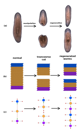
that should be injected by manual calculation of the rectangular region coordinates in the simulation where the cells are present. After the injection of Lysis, simulations consisting of two worm fragments are advanced 200 steps prior to evaluating the emergent outcomes.

As shown, the manual set up of even a simple experiment can be time-consuming. In order to simulate the many experiments described in the literature, some level of computational automation should be achieved.

1.4 Tools

1.4.1 Computational Platform and Evolutionary Search

CellSim, the computational platform used in this work, acts as a digital wet bench and allows simulation of a variety of di erent scienti c experiments performed on planaria worms, like the one shown in Figure 1.1. CellSim includes a development engine where the primary computational unit is a virtual cell. Each cell in the platform acts as an autonomous agent and is capable of growing, dividing, dying, and regulating metabolic and genetic networks in response to changes in its local environment. To model the cells complexity, each cell can contain several subunits capable of in-cell communication. Subunits provide spatially distinct internal cell chemistry, facilitate cell growth and division, and provide internal and arbitrary cell shaping capability. In this work, atworm morphologies are simulated with a at sheet of genetically identical, autonomous cells, each consisting of one and two cellular subunits. Three indicator resources (hCell, iCell, and tCell) have been introduced to

Figure 1.2: CSGA evolutionary search ow.

CellSim to represent three main regions of a planaria worm, head, trunk, and tail, respectively. Figure 1.1b shows worms simulated using one subunit cells.

In addition to the development engine, the CellSim computational platform in cludes an evolutionary search engine and selection to facilitate the discovery and validation of planarian regeneration models. During the evolutionary search, CellSim simulates an experiment and returns the cellular outcome of the experiment. The
cellular outcome produced by the simulation platform is compared to the target morphological outcome, yielding a tness value to guide the evolutionary search.

The ow of the evolutionary search performed in conjunction with the simulation platform is shown in Figure 1.2. In the gure, the simulation starts o with an intact worm consisting of head (blue), trunk (yellow), and tail (purple) regions. The worm is simulated for 200 steps to reach a stable metabolic state, and then a transverse cut is performed on the worm. The simulation runs for 200 more steps and the simulation outcome of the morphology is evaluated against the target outcome. In the gure, the target outcome is evaluated against a morphology represented as a Planform database graph. However, the exibility of CSGA does not require the target morphology to be of a particular representation. For example, the difference distribution tness function uses a hand-crafted CellSim simulation snapshot as the target morphology.

1.4.2 A Database for Storing Planarian Experiments

The automation of search for the models of planarian regeneration that t all the planarian experiments reported in the literature would be intractable without automatic access to the described experiments and outcomes. Lobo et al. developed a graph ontology for e cient storage, search, and mining of the regenerative experiments performed on planaria worms [24]. Planform formally encodes a wide range of morphologies, manipulations, and experiments. Instead of relying on imprecise and ambiguous natural language descriptions of worms, Planform formalizes planarian phenotypes using labeled mathematical graphs. A graph is an abstract representation of a set of objects that can be connected to each other via edges. In Planform formalism, the graph nodes represent body regions, while the edges describe the adjacency between two regions. Nodes and edges can store geometric characteristics of the worm anatomy, such as body region type, overall shape and size of regions, the rotation of organs, and other properties.

The planarian wild-type morphology is characterized by a long at body consisting of three main regions: head, trunk, and tail (Figure 1.3a). The head region is most anterior and contains two brain lobes and two eyes; the trunk contains the pharynx (a muscular tube used for both food intake and waste disposal); the tail region is the most posterior. A nerve cord runs along the length of the worm, starting in the brain lobes and ending in the tail.

Figure 1.3: A wild-type planarian organism (a), along with its graph representation (b) in the Planform software tool.

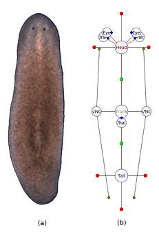
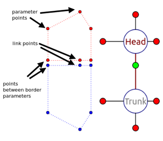
Following the formalism, Figure 1.3b shows a schematic representation of the morphology in Figure 1.3a, in which the circles denote vertices and red lines denote edges. Each vertex is labeled with the region type it represents, such as head, trunk, and tail. Region locations are stored as edge labels containing the distance, angle, and location of the border between the two connected regions (represented as green dots in Figure 1.3b). Region shapes are abstracted as a list of numerical parameters that represent the distance between the center of the region and its border in a speci c direction (red dots connected to region vertices in Figure 1.3b). Non-connected regions have four parameters corresponding to the right, anterior, left, and posterior directions; regions connected to one region have three parameters corresponding to +90, +180, and +270 degrees with respect to the direction of the edge (head and tail regions in Figure 1.3b); regions connected to more than one region have a parameter for each bisector of every two consecutive edges (trunk region in Figure 1.3b). The formalism can also represent organs, such as a ventral nerve cord, brain, and eyes, as shown in Figure 1.3b; however, the organs are beyond the scope of this work and will not be discussed here.

In addition to the formalism describing the shapes of planarians, the Levin lab introduced formalism for experiment manipulations. The formalism includes four basic manipulation types: remove (an area of the organism is cut out and discarded), crop (an area of the organism is cut out and the rest is discarded), and join (two worm pieces are grafted together). The manipulations performed in an experiment are abstracted as a mathematical labeled tree, in which the nodes represent basic manipulations and the edges connect manipulation outputs and inputs. The leaves of the manipulation tree represent the morphologies used to start the experiment, while the root of the tree presents the morphology whose regenerative capabilities are tested. Figure 1.4 shows a simple experiment tree consisting of three nodes- one is the starting morphology, and the rest are cuts performed on it. The root of the tree is a morphology whose head and tail regions have been removed. The above described formalisms for experiment manipulations and planarian shapes are used as a schema for PlanformDB. PlanformDB is a database that has been created to store all experiments performed on atworm planaria published in the literature. The population of the Planform DB is currently underway. To facilitate the use of the formalism and the Planform database, Lobo et al. designed and implemented a software tool called Planform (Planarian formalization). Planform software provides an intuitive GUI where users can view the experiments and morphologies

Figure 1.4: A manipulation tree for an experiment involving removal of the head and tail regions.

encoded in either the centralized database of planarian experiments published in literature or with personal databases created by any user. Despite the exibility of Planform software, it does not provide any APIs to access the database experiments and morphologies programmatically. As a part of this thesis, an API to read and write to the database of planarian experiments is developed.

1.4.3 A Sample Regeneration Model

One of the most interesting properties of planaria regeneration is their ability to robustly regenerate head and tail regions in the correct orientation relative to the starting worm. The Andersen lab set to explore the problem of how the worm is able to determine whether the head, or tail (or both) is missing, and the proper location for regeneration of the missing parts- without the added complexity of regenerating other structures, such as eyes, intestinal tract, and nerve cord. To explore this problem, and to facilitate the evaluation of di erent tness metrics, a simpli ed model of planarian regeneration has been hand-designed by the Andersen lab that utilizes cell polarity as the basis for regeneration of the correct anterior and posterior ends. The polarity of each cell is established using hPole and tPole resources that the cell accumulates in opposite ends. The model is composed of a at sheet of 168 cells arranged as a rectangular abstraction of an intact worm. Every cell in the polar model is autonomous but is controlled by an identical genetic network and each cell knows exactly where the head and tail (north and south) regions are located in relation to itself due to its internal polarity. Head, trunk, and tail regions in this model are represented by cell state indicator molecules, hCell, iCell, and tCell, whose homeostasis is ensured by a set or promoter genes.

The polarity model is capable of regenerating tissue damage from simple transverse cut experiments. In response to a simulated cut, a Regeneration signal activates a Regeneration pathway, which simultaneously promotes head and tail development responses. The cut site only exposes one end of a cell to pick up the Regeneration signal, dependent on the polarity of the cell in relation to the damage. The exposed portion of the cell is then stimulated to regenerate either head if the exposed end is pointing north or tail if the exposed end is pointing south.

CHAPTER 2

GRAPH EDIT DISTANCE FITNESS FUNCTION

2.1 The Graph Formalism for Comparing Worms

The challenge of automating the search for mechanistic interpretations of planarian regeneration is made more tractable by the database and formalism developed to describe experiments and their outcomes [24]. Automating the search process using this data requires the ability to compare the results of simulation data to the graph representations stored in the database. The conversion of the cell simulation results into a graph representation has been chosen for a number of reasons, including increased exibility. For instance, an alternative modeling platform can be introduced or substituted for CellSim with minimal changes as long as its output can also be translated into this graph formalism. More importantly, many methods exist for operating on, transforming, and comparing graphs, which can be included as part of the fitness evaluation step of an automated evolutionary search. Among those are the algorithms designed to measure the similarity between two graphs. From the comparison algorithms, the graph edit distance algorithm is the most exible and powerful and was chosen as it deals with structural errors and any type of graph node and edge labels [32].

The graph edit distance is defined as the minimum number of distortions required to transform one graph into another graph. These distortions are referred to as graph edits, where each edit has a de ned cost associated with it [32]. A particular sequence of edit operations required to transform one graph into another is called an edit path, and the total cost of the edit path is its graph edit distance. Graphs that are similar to each other typically have small edit distances, whereas dissimilar graphs have large edit distances. The cost of each type of graph edit operation varies and is dependent upon the perceived severity of the operation. For example, the deletion of a node from a graph is generally viewed as having a higher cost than a node parameter change.

Thus, the graph edit distance can be used as a similarity measure to compare and order individuals within a population, and thus serve as a metric within a fitness evaluation to guide the evolutionary search process. Dr. Daniel Lobo adapted the graph edit distance algorithm to be used with the planarian formalism graphs in PlanformDB [24]. The graph edit distance costs used in the algorithm implementation are described in Table 2.1. The penalties are most severe when differences exist between region numbers and connectivity than for region size and linkage parameters.

Table 2.1: This table presents the graph edit costs used for graph edit distance calculations in this manuscript.

As a part of this thesis, the C++ implementation of graph edit distance algorithm has been incorporated with the CellSim simulation platform. Since the simulation platform is implemented in Python, a Python to C++ interface has been developed to pass the Python graph objects as parameters to the C++ graph edit distance library. The interface between the simulation platform and graph edit distance library uses the ctypes foreign function library, which includes C compatible database types and capability of calling functions inside DLLs and shared libraries.

2.1.1 Design of a Connected Component Analysis Algorithm to Convert Cell Simulation Output into Graph Representations

Planaria in the CellSim platform are composed of a collection of discrete cells rather than interconnected regions. Thus, a rst step to deriving a graph-based representation of the cell-based planaria is to translate the cells within a simulation snapshot into discrete regions, and to determine which regions are connected to each other. In order to do this, an algorithm that uses a connected component analysis approach derived from similar methods used in computer vision and document analysis has been developed [4]. The algorithm first iterates through all the cells in a snapshot and assigns each cell a region type (e.g., head or tail). The assignment of cell type can be complicated, examining many different factors for each cell, or can simply depend on the molecular concentrations of some user-de ned indicator resources associated with a particular cell. Three resources, hCell (head), iCell (trunk), and tCell (tail) have been defined to serve as cell-state indicators in this study. For this work, a simple approach is used where a cell is assigned to a region type based on the highest total concentration of each indicator resource. For example, a cell is assigned a trunk

Figure 2.1: The assignment of a cell to a state depends on the molecular concentrations of cell-state indicators. The di erentiate state of cells are color-coded to enable visual distinction of cells and the composition of a region: head (blue), trunk (yellow), and tail (purple). Within a given cell, the location of a given resource can be distributed between the internal compartment (e.g., cytosol) and the surface (e.g., membrane). Concentrations of representative resources inside (I) and on the surface (S) are provided. In this example, both Cell 1 and Cell 2 are assigned to a trunk state and Cell 3 is assigned to a trunk state, since the concentrations of the indicator molecules (iCell and tCell, respectively) for these states are the highest.

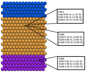
state if its concentration of iCell is greater than hCell and tCell, as shown in Figure 2.1. The approach of assigning a cell to a region based on the highest concentration of an indicator resource is a simpli cation of reality, since many more factors may go into di erentiation of a cell in an organism. Chapter 3 examines a more complex way of evaluating a cells region type.

After calculating cell type, the algorithm must determine all of the spatially cohesive regions of cells sharing the same type using connected component analysis. The connected component analysis algorithm (Algorithm 2.2) starts with a call to the Process Connected Components function with a simulation snapshot as a parameter. A simulation snapshot is a complete description of a particular step in a simulation; this includes a list of all cells, including cell contents, resources, and locations.

ProcessConnectedComponents(snapshot):
list = new list of connected components
for each unprocessed cell c in snapshot
comp = new connected component
add c to comp
set c as processed
GatherConnected(c, comp, snapshot)
add comp to list
for comp in components:
calculate parameters for comp
GatherConnected(c1, comp, snapshot):
for each unprocessed cell c2 in snapshot
if c1 and c2 are connected:
if c1 and c2 are not of the same type:
mark c1 and c2 as border cells
else:
add c2 to comp
set c2 as processed
GatherConnected(c2, comp, snapshot)

Figure 2.2: Pseudocode for connected component analysis recursive algorithm to separate a list of cells taken from the simulation snapshots into discrete morphology regions.

The Process Connected Components function iterates through all cells and calls the Gather Connected function for each unassigned/marked cell.

The Gather Connected function recursively collects and marks all other cells in the snapshot that belong to the same spatially cohesive region as the starting cell. A cell is defined to be in the same spatially cohesive region as the starting cell if it is of the same type as the starting cell and is either connected to the starting cell or to
some other cell already determined to be in the starting cells region. Two cells are considered connected if the Euclidean distance between them is below a user-specified threshold. Additionally, if two cells are close enough to each other to be considered connected, but are assigned to di erent regions because they are of di erent types, those cells are identi ed as border cells. Border cells are used to determine which regions are linked to each other.

Once each cell in the snapshot is assigned to a speci c region, links between regions are calculated. The algorithm determines how many neighbors each region is connected to using the border cells found during the recursive process in Algorithm 2.2, and creates links between the connected regions. Two regions are be considered linked if they share border cells.

By the graph formalism, each link between regions is parametrized by the distance between the connected regions centers, the angle of the link measuring its tilt relative to the x-axis, and the location along the link where the two regions meet. The number of parameters for a region depends on the number of links it has. A component parameter is de ned as the Euclidean distance from the center of a region to a region border in a speci c direction. The center of a region is calculated by averaging the spatial centers of every cell in a particular region. The border of a region is calculated by nding the furthermost cell in a specific direction.

The connected component gathering algorithm allows the cell-based representation of the worm to be converted into a graph, and this graph can be subsequently compared to a target graph pulled from the Planform database. The result of the graph-to-graph comparison is used as a tness value to guide the genetic algorithm search process.

2.1.2 Graph Edit Distance as a Fitness Function

Since the GA is designed to evaluate fitness values in the range of 0.0 to 1.0, the graph edit value cannot be used by itself to measure the fitness of simulation outcomes, and thus is converted as shown in Equation 2.1.

fitness =5000 by (distance + 5000) (2.1)

Initially, the simple inverse function of 1/(graph edit distance) was used to obtain the GA tness values. However, the tness function values in such cases tended to be very small even for relatively similar graphs due to sensitivity caused by the large edit penalties in Table 2.1.

To come up with an equation for converting graph edit distance values to tness values that is capable of producing more intuitive tness values, several morphology graphs were evaluated using the graph edit distance tness function. The graph edit distance value for the tested graphs was converted into a value between 0.0 and 1.0 using Equation 2.1 with di erent constants in the range between 1 and 10000. Constants above 10000 were excluded from the evaluation on the basis of generating high fitness values for individuals with morphologies very dissimilar to the target.

Table 2.2 shows the graph edit distance and the tness values produced for 13 different graphs (ID-1 though ID-13) compared against the target graph (ID-0). The third column in the table displays graph edit distance values for graphs, while the columns following it present the tness values produced by using constants in the column headers.

Table2.2: Evaluation of conversion equations to generate fitness values from graph edit distance values. The first row presents the data for the graph of the target individual. The first and second columns of the table show the I D and the image of the morphology graph. The third column presents the graph edit distance value
obtained from comparison of the graph against the target graph using graph edit distance algorithm. The fourth through the ninth column show the fitness value produced by plugging in the constant in the column header into Equation 2.1.

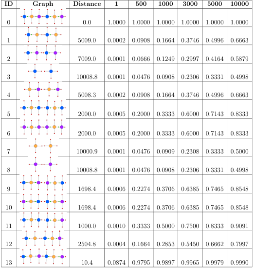
The constants of 500 and 1000 both produced very low values to the individuals tested, and thus were not optimal for the fitness conversion equation. The constant of 10000, on the contrary, yielded tness values that were too high and did not maximize the differences between tness values. In the last column of Table 2.2, which corresponds to the constant of 10000, the tness values range from .49 to 1.0, which is not a very large tness range for the individuals tested.

The constants of 3000 and 5000 could both potentially perform well in the evolutionary search, since both of these constants have a big fitness range. However, for some graphs, the constant of 3000 produced fitness values lower than we would otherwise intuitively assign and that would be better at guiding the evolutionary search. Consider, for example, an individual with an ID of 12. The first half of the individual does not have a tail regenerated, while the second half has regenerated its head region. This individual has shown that it is capable of regeneration and can successfully regenerate a head region. Even without the tail regeneration in place, intuitively this individual should not receive a fitness as low as .54, as yielded with the constant of 3000. The fitness of 0.66 for this individual produced using the constant of 5000 seems appropriate and intuitive. Therefore, the constant of 5000 was chosen for an equation to convert graph edit distance values into fitness function values as it produced an appropriately large range of fitness values and assigned most-intuitive fitness values.

CHAPTER 3

OVERLAY FITNESS FUNCTION

3.1 Comparing Two Morphologies by Overlaying a Graph with a Blob of Cells

The graph edit distance evaluator is a very exible tness function, since the graph formalism can be used in simulation platforms other than CellSim. However, the graph edit distance evaluator may in some instances fail due to the coarse grained nature of how it determines cell region type. The assignment of a cell to a region is a very complex question, since many factors determine whether a cell belongs to a particular region. The implementation of the component gathering algorithm uses a very simple approach for determining the cells region relation. This approach may not work well when a cell has the potential of becoming the sought-for region type. For example, a cell that has hCell concentration of 0.1 and iCell concentration of 1.0 can potentially become an hCell, but this cell will be assigned to a trunk region. This cell may get penalized by the graph edit distance evaluator if it expects the cell to be of type head. As an alternative to the graph edit distance evaluator, the overlay distance tness evaluator has been developed. In contrast to the graph edit distance evaluator, the overlay evaluator rewards a cell that is close to becoming the expected region type, and will not penalize the cell as much.

The overlay tness function calculates the best t of a morphology graph to a cell-based model as shown in Figure 3.1. To create an overlay, the graph is scaled so that the graph ts inside of the cellular morphology and matches the width of the height of the morphology. For each cell in the cell-based morphology, the closest graph region of the overlayed graph is found. The cell gets assigned a sub fitness based on how close the cell is to becoming the expected graph region.

Figure 3.1: In this example of overlaying a cellular morphology with a graph morphology, the cellular morphology consists of three regions, head (red), trunk (blue), and tail (green), while the overlayed graph only has a head and a trunk. When the graph is overlayed with the cellular morphology, some of the cells do not match the type of the overlayed graph (colored in black).

Classic experiments on planaria worms involve cuts separating a whole worm into several parts. For example, if a transverse cut is performed on a planarian, as shown in Figure 1.1, two cut pieces are expected to regenerate into complete worms. Therefore, to evaluate the e ectiveness of the regeneration model, each of the regenerated pieces needs to be compared to the target. Algorithm 3.2 shows pseudocode for the overlay di erence evaluator. The Over lay Difference Evaluator function of Algorithm 3.2 accepts two parameters: the cut up worm, represented as a cellular snapshot in CellSim platform, and a list of graphs to be over layed with the cut up pieces. The cellular snapshot does not keep track of cuts performed on the worm, and stores the cells of the cut up pieces in a single

OverlayDifferenceEvaluator(snapshot, graphList):
Convert the cellular snapshot to blobs
Sort blobs based on their centers
Let cellSellsubfitnessSum = 0
For each blob:
Convert corresponding graph from graphList into 2D lines
For each cell in the cellular morphology snapshot:
Find closest graph line to the cell
Set expectedRegion to the region of closes the graph line
Calculate the cell subfitness
Add the cell subfitness value to cellSellsubfitnessSum
return cellSellsubfitnessSum / number of cells in a snapshot

Figure 3.2: Overlay difference fitness evaluator

list of cells. Since an overlay needs to be calculated for each cut up piece, or blob, the cells in the snapshot cell list get separated into lists of blob cells. Each blob in the blob list is matched with a corresponding graph in the list of target morphology graphs provided by the user. Knowing the exact order of the blobs, the user can provide the correctly ordered graph list constituting the target morphology, so that the first blob is compared against the rst graph, and so on. Providing a list of graphs instead of one graph with several subgraphs was required because the graph ontology of PlanformDB does not give any information about relative location of disconnected
subgraphs. To calculate the overlay between a cellular-based blob and a graph, the graph needs to be converted to 2D lines as discussed in Section 3.2. The closest 2D line to a cell dictates what region a cell should be in order to match the graphs region.

A sub tness value between 0.0 and 1.0 is calculated for each cell measuring how far the cell is from becoming the expected region as shown in Equation 3.1. A cellular sub fitness is calculated by measuring the ratio between the concentration of the target molecule and the maximum concentration of an indicator molecule in a cell.

subfitness = max(conc(target mol)by conc(mol with maximum concentration) 1) , (3.1)

The final fitness of the model in the overlay evaluator is calculated by dividing the sum of sub fitness values for every cell in the organism by the number of cells.

3.2 Graph-to-Line Conversion

To calculate an overlay of a graph to a cellular blob, the dimensions of the graph and the blob need to match. In the CellSim simulation platform and Planform graph formalism, the coordinate systems are arbitrary and carry no spatial meaning. For example, in the database and the simulation platform, the distance of 1 can mean the distance in millimeters, centimeters, etc. Due to the lack of spatial meaning of the coordinate systems, cellular and graph morphologies can be scaled in order to be matched and compared to each other without any loss of information. The graph formalism used to encode morphologies in the experiment database
stores morphology regions as graph nodes with parameters describing the general node shape. Graph node links contain information about how far away connected nodes are from each other and what their angle position is. For overlay to cover as much of the cellular worm as possible, the graph is expanded geometrically through conversion of the graph nodes into connected lines tracing the silhouette of the graph. The graph formalism does not provide xy coordinate locations for region nodes and links. So before the lines for regions can be computed, the graph nodes, parameters,

and links need to be projected into an x-y coordinate system. The algorithm randomly takes a node in the graph and assigns its center to the (0,0) coordinate. The coordinates for the parameter points de ning the shape of the node are calculated based on the nodes center. Using the rst nodes center coordinate and the distances to the nodes this node is connected to, the algorithm recursively assigns the coordinates to the rest of the nodes in the graph. Once the graph nodes, parameters, and links have been projected into the x-y coordinate system, the points defining the silhouette of the graph are computed.

The points in the graph-to-line conversion algorithm can be of three types: parameter points, link points, and points between border parameters. Figure 3.3 shows a sample graph with the three point types indicated. In the graph formalism, a parameter for a region indicates the distance from the region center to the parameter point in a speci c direction. Parameter points lie at the end of the parameters. Link points lie on a border line that connects the centers of two nodes. For each parameter point on a border between two regions, an additional point is calculated to help define a more accurate shape of the worm for the overlay. In the gure, it is called a point between border parameters. The calculated points for a node get connected into lines and can be used to create the overlay.

To ensure that the graph converted into lines matches the dimensions of the cellular blob, either the cellular morphology or the graph can be scaled. Cellular morphologies consist of a large number of cells, and scaling of a cellular morphology requires scaling to be performed on every cell. For the purpose of e ciency, the scaling was chosen to be performed on the graph morphology instead of the cellular morphology. The graph scaling factor is calculated by taking the minimum between the blob-to-graph height ratio and the blob-to-graph width ratio. This approach

Figure 3.3: Sample conversion of a two-node morphology graph into lines. Three point types calculated during the conversion algorithm are indicated.

guarantees that the graph is within the blob, no matter whether it was generally bigger or smaller than the blob before the scaling operation was applied. Once the scaling has been performed, and the width and height of the graph match those of the cellular blob, the nal step of the conversion is to match the centers of the two representations. Center matching is done by performing a transform on each 2D point in the converted graph. The graph converted into lines that matches the dimensions and the center of the cellular blob can be used to calculate the overlay fitness value.

CHAPTER 4

DIFFERENCE DISTRIBUTIONS FITNESS FUNCTION

4.1 Comparing Two Morphologies by Calculating Difference Distributions of Their Resources

While abstracting the worm morphology into regions allows a very exible means of comparison between the simulation platform outputs and the target PlanformDB morphology, the graph representation may be too coarse-grained in certain instances as discussed in Chapter 2. As an alternative to abstracting the cellular representation of the worm in the simulation platform, the simulation outcome can be viewed as a multidimensional vector, consisting of multiple features, such as molecular concentrations and individual cell locations. Vectors for the simulation output and the target may vary signi cantly, and so exible comparison algorithms are needed to calculate the differences between multidimensional vectors describing two distinct worms.
The problem of matching two multidimensional vectors is common in computer vision where the similarity between 3D shapes is measured. Most 3D models tend to have missing, wrongly-oriented, intersecting or disjoint polygons [34]. Since most 3D comparison algorithms rely on standarized 3D models with some sort of required metadata, the traditional 3D matching methods cannot be used for comparing arbitrary 3D shapes. Moreover, these traditional algorithms cannot handle shapes containing holes in the surface. To mitigate the limitations of traditional shape comparison algorithms, Osada et al. proposed an algorithm to compare arbitrary 3D models using shape distributions [34]. Osada et al.s algorithm calculates a signature for each 3D shape by sampling from a shape function, which measures
geometric properties of a 3D model. For example, the samples for a shape can be gathered by calculating distances between 3D points in the shape and then normalized into a distribution. The normalization of a shape distribution allows Osada et al.s algorithm to be translation, rotation, and size-invariant. To compare two 3D shapes, Osada et al.s algorithm calculates the di erence between the normalized distribution signatures for the shapes.

Just like 3D shapes, simulation outcomes of planaria regeneration models are multidimensional objects that may have missing structures, such as cells, genome regulatory regions, or metabolic equations. Simulation outcomes may also be rotated differently than the target due to the experiment setup, and thus signi cantly vary from the target in a structural, though not necessarily in an functional, way. In this work, Osada et al.s di erence distribution algorithm has been incorporated as a GA tness function that can compare simulation outcomes to the target outcome.

The di erence distribution tness evaluator computes a statistical signature, or a difference distribution histogram, for the internal state of the worm by considering concentrations of speci c molecules and locations of individual cells. Fitness value of the simulation outcome is calculated by comparing the di erence distribution histograms of the simulation outcome and the target outcome. Algorithm 4.1 shows how the distribution signature can be calculated. The main function of the algorithm (distribution) rst takes samples (takeSamples) and then creates the normalized di erence distribution histogram for the simulation outcome (createDistribution).

In the default implementation, distances between two points are taken exhaustively for every pair of cells. The samples gathered include distances between the cellcenters of mass and molecular concentrations of cells. For each sample, the distance between two cells is computed by calculating the sum of squared di erences of cells locations and molecular contents (processCells).

As an alternative to exhaustive sampling, stochastic sampling can be specified in which only a certain number of measurements are taken for randomly chosen cells. To get a more precise distribution of the simulation outcome, a subunit-to subunit distance can be computed. The subunit-to-subunit di erence processor uses the process Cell Sub units function, which iterates over all subunits in two cells and compares the subunits locations and molecular contents. The sub unit-to-sub unit processor is more compute intensive, but it also allows a more accurate representation of the simulation models shape and location of molecular contents.

The obtained samples are used to construct a di erence distribution histogram by counting how many samples fall into each of B xed size bins (calculateDistribution in Algorithm 4.1). The number of samples that falls in each bin is normalized by dividing the sample count for a bin by the total number of samples taken. Once difference distributions histograms for the simulation outcome and the target are constructed, the dissimilarity between histograms is computed. As shown in Algorithm 4.2, absolute di erence is computed for every matching value in each bin, yielding an array of absolute di erences. The values in this array are summed into the variable di erenceSum, and this value is normalized using Minkowski LN norm [34].

distribution():
takeSamples()
createDistribution()
takeSamples():
for cell1 in cells:
for cell2 in cells:
processCells(cell1, cell2)
processCells(cell1, cell2):
sum = 0;
sum += calcSquaredDifference(cell1.x, cell2.x)
sum += calcSquaredDifference(cell1.y, cell2.y)
sum += calcSquaredDifference(cell1.z, cell2.z)
for each molecule mol:
sum += calcSquaredDifference(
mol concentration in cell1,
mol concentration in cell2)
add sum to the list of measurements
calculateDistribution():
let binCounts be an array of size B
let measurementCount be the size of measurements
for each measurement in measurements:
binCountIndex = calculate the bin for the measurement
binCounts[binCountIndex]++
normalize each binCount in binCounts by measurementCount
Figure 4.1: Distribution calculation using using a cell processor

absoluteDifference(a,b):
return |a-b|
calculateFitness()
//get a list of absolute differences of two bins
absoluteDifferences = map(absoluteDifference, bins1, bins2)
differenceSum = sum all the absolute differences in the absoluteDifferences
return 1- differenceSum/2.0

Figure 4.2: Fitness calculation using di erence distributions

As an alternative to Minkowski LN norm, distribution histograms can be compared using any standard methods, such as Kolmogorov-Smirnov distance, Kullback-Leibler divergence distances, Bhattacharyya distance, and others [34].

CHAPTER 5

EXPERIMENT DATABASE READER AND WRITER

The Plan form DB of planarian experiments is an invaluable tool for searching the experiments reported in the literature. To provide access to PlanformDB and the ability to add new experiments into the database, the Levin lab implemented an executable GUI program called Planform that allows users to view, search, and manually edit database morphologies and experimental manipulations [24]. Being the sole access point to the database, Planform allows for only manual modi cation of the database and does not provide APIs to read and write to the database programmatically. Without programmatic access to PlanformDB, utilizing the database in the evolutionary search and the simulation platform is ine cient. Running experiments, injecting worms with Lysis, and creating cellular morphologies by injecting head and tail indicators would be performed manually and thus would be time-consuming. To alleviate this problem and allow automatic retrieval of information pertinent to planarian experiments, a database reader and writer that can program matically access and manipulate Planform DB have been created. The database reader and writer represent the SQLite database entities as Python classes that can be accessed and manipulated by CellSim and CSGA. Figures 5.1 and 5.2 show the UML diagrams for the Python classes that represent a database morphology and an experiment, respectively. The structure of these classes reflects the database schema of PlanformDB described in Section 1.4.2.

5.1 Experiment Database Reader of Morphologies and Experiments

Just like in PlanformDB, the main Python class representing a planarian is called Morphology, as shown in Figure 5.1. Each morphology consists of interconnected regions (class Region) such as head, trunk, and tail. A region knows exactly what other regions it is connected to by maintaining a list of region links (class RegionLink). A region also knows what organs are contained within it, such as spot organs (eyes, brain lobe, pharynx) and line organs (ventral nerve cord). The current work did not deal with morphologies containing organs; however, the implementation of the classes was designed so that in future studies organs can be incorporated into the the evolutionary search.

The main Python object pertaining to a PlanformDB experiment is represented by the Experiment class, as shown in Figure 5.2. An Experiment object knows what instance of PlanformDB it comes from as well as the name it is encoded with in the database. Each Experiment object stores a tree of manipulation actions (class Manipulation) that are performed on a worm as a part of the experiment. A Manipulation object keeps a reference to the root of the manipulation tree, where each tree node is represented as a ManipulationAction object. There are four types of manipulation actions speci ed in the PlanformDB schema: crop action (class CropAction), remove action (class RemoveAction), join action (class JoinAction), and

Figure 5.1: UML diagram for the Planform database morphology.

morphology action (class MorphologyAction). The four action classes in Python were implemented to inherit from the base Manipulation Action class, since they all share attributes, including the name of the manipulation and the reference to the child manipulation action. CropAction and RemoveAction objects store a list of points representing an area that should be respectively cropped or removed from a planarian morphology. The JoinAction represents the grafting of two manipulation action subtrees, while the MorphologyAction simply stores the reference to the Morphology object on which the manipulations are to be performed. Python objects representing planarian morphologies and experiments performed upon them can be obtained by directly communicating with the Planform SQLite database. To this end, a Python interface for reading and writing to the experiment database was implemented. Figure 5.3 shows a UML diagram for the database reader capable of extracting Planform experiments and morphologies. The modules are adapted to call SQLite queries on PlanformDB using sqlite3 Python library. In Figure 5.3, DBReader class acts as the generic interface to the database that can

Figure 5.2: UML diagram for the Planform database experiment.

connect to an SQLite database and call SELECT statements on it to retrieve values from a speci ed table. DB Experiment Reader and DB Morphology Reader classes use the DB Reader class to access the PlanformDB and extract values pertinent to the experimental manipulations performed on planaria as well as planarian morphology graphs. To extract a planarian morphology from PlanformDB, the DBMorphologyReader class calls the processMorphology function, which takes morphology name or ID as a parameter. This function creates a blank Morphology object and calls the processRegions function, which in turn creates an initially empty list of morphology regions and iterates over the regions in Planform DB, creating Python Region objects and adding them to the region list. As each Region object is created, the process Region Params is called, which reads parameters representing the general shape of planarian region morphology.

Figure 5.3: UML diagram for the Planform database reader.

DBMorphology Reader provides the capability to automatically retrieve morpholo gies to be used as targets during the CSGA evolutionary search. Since in addition to the morphology descriptions, Planform DB stores experiment manipulation descriptions, it is crucial to provide capabilities to read the experiment manipulations as Python objects to fully automate the evolutionary search. The DB Experiment Reader class is responsible for reading an experiment from Plan form DB and constructing an Experiment object that can be eventually used on a cellular morphology in the simulation platform. The functions used by the experiment reader are shown in Figure 5.3. Just like the DB Morphology Reader, the DB Experiment Reader gradually creates the Python objects representing an experiment (process Experiment), a manipulation (process Manipulation), a tree of manipulation actions (process Action Subtree), as well as the specific manipulation actions (process Morphology Action, process Remove Action, process Crop Action, process Join Action). The created Experiment object can then be used by the manipulation applicator described in Chapter 6 to perform the Plan form DB experiment on the cellular morphology from the simulation platform.

5.2 Experiment Database Writer of Morphologies

During the evolutionary search, large numbers of unique individuals are generated. Even though the individuals produced by the genetic algorithm are automatically evaluated by the tness function and selected for further generation cycles, extra human checking may be needed to examine the progress of the evolutionary search. Since graphical representation of planarian morphologies is a lot more user-friendly than the XML les describing regeneration models in CSGA and CellSim, it is deemed useful to save unique individuals discovered by the GA into the PlanformDB. To this end, a Python module has been designed to write morphology Python objects to a user-specified database. Embedded in the evolutionary search, this module automatically saves unique mor phologies to a database tied to the currently performed search.

Figure 5.4 shows the UML diagram of the database writer class (class DBMorphol ogyWriter). The writer class contains a reference to a Python sqlite3 cursor object that references an instance of the PlanformDB and allows it to send simple SQLite queries. The top level functions of the writer provide the capability to insert and

Figure 5.4: UML diagram for the Planform database writer.

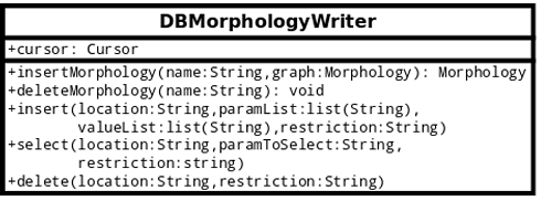
(1) SELECT Id FROM Morphology WHERE Name=Wild type
(2) INSERT INTO Morphology (Id, Name ) VALUES
(
(SELECT max(Id) FROM Morphology )+1,
Wild type
)
(3) DELETE FROM Morphology WHERE Id=17
Figure 5.5: Sample SQLite queries to call to PlanformDB.

delete morphology graphs with specified names to and from the database. These two functions are implemented using three basis functions, insert, select, and delete, which in turn execute the SQLites basic INSERT, SELECT, and DELETE commands. To demonstrate the usage of these functions, consider SQL commands depicted in Figure 5.5. Command (1) gets the ID of the morphology, which has the name Wild type in the Planform database. Command (2) inserts a new row into the morphology table with the name of Wild type and an ID, which is one higher than the biggest ID in the table. To run queries (1)-(3), select, insert, and delete functions defined in Figure 5.4 get called with the parameters shown in Figure 5.6.

(1) select(
(2) insert(
(3) delete(
location = “Morphology”,
paramToSelect = “Id”,
restriction = “WHERE Name=” + “Wild type” + “”
)
location = “Morphology”,
paramList = “Name”,
valueList = [Wild type],
restriction = “”
)
location = “Morphology”,
restriction = “WHERE Id=” + str(17) + “”
)
Figure 5.6: Sample calls of Python database writer functions.

CHAPTER 6

AUTOMATED EXPERIMENT EXTRACTION AND
APPLICATION

The CellSim simulation engine provides a simple, easy-to-use graphical tool to select and manipulate cells as shown in Figure 6.1. With this tool, a user can inject various resources, such as Lysis and region indicators, into selected cells.

The CellSim GUI software works great for manually manipulating individual worms; however, to perform such manipulations on a large number of individuals, as is required by the evolutionary search, an automated setup is required. The experiment setup in CSGA involves design and implementation of a custom Python fitness evaluator to select desired cells for manipulation and perform the experiment on them during the simulation run. Typically, a custom evaluator only works for the experiment for which it is written. In order to change the experiment or the manipulated morphology, the code for the custom Python evaluator has to be hand-adjusted or sometimes entirely rewritten. This process is not only ineficient but also prone to human errors. To alleviate the problem of hand-adjusting code for every new experiment and to automate the manipulation application on large populations of cellular morphologies in the simulation platform, a Python module has been created that provides translation of the experiment setup encoded in PlanformDB into the experiment setup in CellSim.

Figure 6.1: The graphical user interface for the CellSim simulation platform.

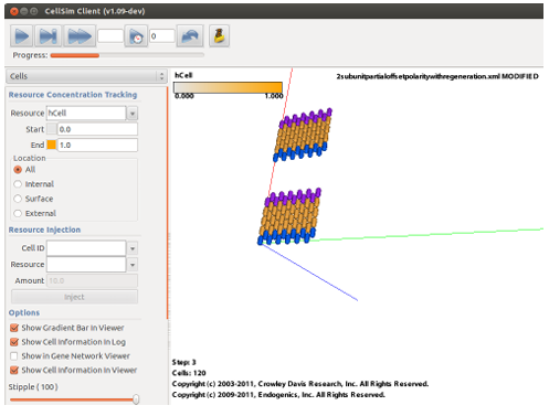
For demonstration of how the developed module automates the experiment application in CellSim and CSGA, consider Figure 6.2. The gure depicts a PlanformDB experiment that involves removal of a rectangular region de ned as a list of four Cartesian points from a wild-type morphology (Fig. 6.2a). In PlanformDB terminology, the points forming the rectangular region of a manipulation action are called action points. To be compatible with the cellular worm, action points get converted into the x, y, z coordinate space of the CellSim simulation platform, and are pasted onto the cellular morphology (Fig. 6.2b). The cells falling inside the rectangular region formed by the action points are then extracted and manipulated according to the experiment specification.

Figure 6.2: Example of applying a Plan form DB experiment manipulation (injection of Lysis) to a cellular model in Cell Sim.

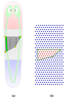
The manipulation application module consists of three classes, each class responsible for a single task. The rst class translates manipulation action points from the PlanformDB coordinate system to the CellSim coordinate system. The second class calculates what cells in the manipulated morphology fall within the area inside the polygon formed by the action points. The third class acts as the coordinator and keeps track of the Planform DB experiment manipulation and the cellular morphology. The UML diagram depicted in Figure 6.3 shows Python classes designed to auto mate the extraction of cells on which the experiment has to be performed. The main
class, Manipulation Applciator, contains a reference to a list of cells represented as Cell Description objects, which constitute the cellular morphology, and a Plan form DB experiment represented as an Experiment object. Manipulation Applicator serves as

Figure 6.3: UML diagram for the Planform DB experiment manipulation applicator.

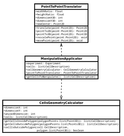
the coordinator for the cell extraction process, and uses two helper classes, Point To Point Translator and Cells Geometry Calculator, to translate action points and extract the cells to be manipulated upon. PointTo Point Translator class scales the points describing the manipulation action in the database to match the scale of the cellular morphology. Given the translated and scaled polygon points and a list of cells, the Cells Geometry Calculator class determines what cells fall inside of the polygon formed by the action points.

manipulationApplicator = Manipulation Applicator(experiment, cells)
cells = manipulationApplicator.getCellsToManipulate()
class ManipulationApplicator:
getCellsToManipulate():
get experiment action points
for each point in points:
PointToPointTranslator.translate(point)
return CellsGeometryCalculator.getCellsInsidePolygon(translated points)
class PointToPointTranslator:
tralslate(point):
rescalePoint(point)
movePoint(point)
rescalePoint(point):
point.x = point.x * width ratio
point.y = point.y * height ratio
movePoint(point):
point = point + worms center location in CellSim
class CellsGeometryCalculator:
getCellsInsidePolygon(polygon):
initialize an empty list as cellsInsidePolygon
for each cell in morphology cells:
if not cellIsOutsidePolygon(cell, polygon):
add cell to cellsInsidePolygon list
return cellsInsidePolygon list
cellIsOutsidePolygon(cell, polygon):
create a ray going from (cell x, cell y) to (infinity,cell y)
for each polygon side of polygon:
if polygon side intersects ray:
return false
return true
Figure 6.4: Pseudocode for extraction of points falling inside the manipulation
polygon formed by action points

Figure 6.4 shows the pseudocode to extract cells falling inside the polygon for a region removal experiment. The pseudocode to extract cells outside the polygon for a crop experiment is very similar and will not be discussed here. The algorithm starts by creating a Manipulation Applicator object, and calling the get Cells To Manipulate function. The get Cells To Manipulate function retrieves action points from the Experiment object and translates them into an x, y, z coordinate system by calling Point To Point Translators translate function. Translation of a point involves re-scaling of the points x and y coordinates by width and height ratios and moving the point by the cellular worms center. The height and width ratios used in point scaling are computed by dividing the cellular worms height by graph worms height and cellular worms width by graph worms width, respectively. An action point is moved to correspond to the Cell Sim worms center since in Planform DB morphologies are always centered at the (0,0) coordinate, while in CellSim the center of the worm may be any coordinate.

Once the action points are translated into CellSims coordinate system, CellsGe ometryCalculator can extract the cells to be manipulated. To get the cells inside the polygon formed by the action points, getCellsInsidePolygon function gets called with a list of translated action points as a parameter. The get CellsIn side Polygon function creates an empty list to store the cells found to be inside the polygon and iterates over all the cells in the morphology, checking if an examined cell falls inside the polygon. If a cell is inside the polygon, it is added to the list. To determine if a cell is inside the polygon, an innite ray parallel to the x-axis and pointing towards positive innity is projected from the cell. The ray is tested against every side of the polygon to check for intersection. If this ray intersects polygon lines an odd number of times, the cell is determined to be inside the polygon, otherwise the cell is outside [16]. The list of cells determined to be inside the polygon is used by the simulation platform for experimental manipulations, such as injection of Lysis.

CHAPTER 7

RESULTS

7.1 Evaluation of the Cellular Snapshot-to-Graph Conversion Algorithm

During an evolutionary search, large numbers of unique individuals are generated and must be evaluated against the target individual encoded in the database. To ensure that converted graph representations are intuitive and to evaluate the use of the graph edit distance metric for ordering individuals in the population, an evaluation of the conversion algorithm was performed. To this end, a number of worms with distinct morphologies was generated by hand using the simulation platform, and their snapshots were converted into graph representations using the conversion algorithm.

The simplest individuals that can be represented by the simulation platform include worms with discrete regions, whereas more complicated morphologies consisting of regions contained within other regions can also exist. Just considering the basic morphologies, the number of individuals that can be formed and the tness landscapes for the genetic algorithm are innite, and therefore the conversion algorithm was tested using simple individuals before considering more complicated morphologies. As shown in Table 7.1, a series of distinct worms (ID 1-13) were generated for comparison with a desired target (ID 0). In each case, the worm representations included two fragments to simulate the state of worms following a single transverse cut. Each worm was generated by injection of the appropriate cell-state resource (i.e. hCell, tCell, and iCell) to create the desired regions within the worm fragments, resulting in di erent permutations of head, tail, and trunk regions. Every test morphology was converted to a graph (Table 7.1, Morphology Graph) using the connected component analysis conversion algorithm. No discordance was found between the graphs generated by the conversion algorithm and those expected upon visual inspection of the simulation output. Thus, the algorithm was working as expected on these simple morphologies. During an evolutionary search, the genetic algorithm needs to compare individuals to the target and reward those individuals that are most likely to turn into the target, that is, possess a reaction network capable of proper regeneration. The genetic algorithm assigns fitness values based upon how evolutionally close the individual is to the target, with closer individuals getting higher tness values. A fitness value of 1.0 is awarded to an individual with a perfect match to the target and is the ultimate goal of a search. Thus, the graph edit distance was calculated between each test individual and the target and those values were converted into a tness value (Table 7.1).
The target individual, when compared to itself, yielded a graph edit distance value of 0.0, because when two individuals are identical, the distance between them measured by the graph edit distance algorithm is 0. Using Equation 2.1 (defined in Section 2.1.2), the distance of 0.0 translates to a fitness value of 1.0, which in our

Table 7.1: Single cut morphology experiment results for simulation snaps hot to graph conversion and graph edit distance comparison

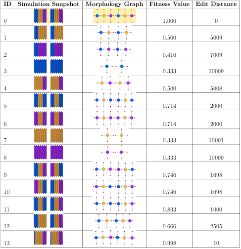
genetic algorithm search indicates the target morphology has been found. Morphology 13 in Table 7.1 is a slight variation of the target morphology, where its heads are several cell layers thinner than the heads of the target, and as expected has the next best fitness value (0.998). In general, high fitness values for morphologies such as
number 13 are expected as their regions are connected and oriented the same as the target. When compared to the target, morphologies that consist of three regions in each worm fragment received higher tness values than morphologies having one or two regions. For example, morphology 6 was rated higher than morphology 4. Again, this is because the graph edit distance costs included a much larger penalty for the deletion of a region than with a change to the type of region.

Conversion of a simulation snapshot into the graph is an O(N2) algorithm where N is the number of cells in an individual. The wild-type morphology had 420 cells, but since the transverse cut removed four rows of cells, the morphologies used in this experiment consisted of 364 cells. The conversion algorithm ran in less than 1.3 seconds for every morphology in Table 7.2. The run time of the graph edit distance calculation grows exponentially with the size of the graphs (number of nodes, or in our case to the number of regions in the two morphologies)[32]. However, since the number of regions in each morphology tested was at most 6, the graph edit distance algorithm finished in less than 1 millisecond for all morphologies.

7.1.1 Cell Connectivity Distance Threshold Effects on Region Determination

Table 7.2: Threshold value inuence on snapshot to graph conversion algorithm

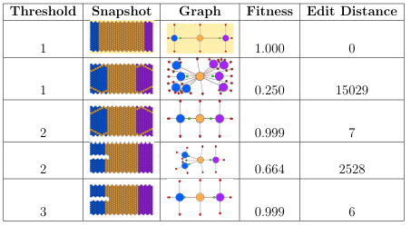
simulation have radii of 0.5 units, the Euclidian distance between two adjacent cells can be as low as one. However, using a very rigid measure for identifying neighboring cells and determining the borders of regions can have dramatic e ects on the graph conversion. For example, consider the morphology of the second individual shown in Table 7.2. In this individual, thin lines of trunk cells dissect the head and tail regions into a number of potentially distinct heads and tails if the borders are considered rigidly. Comparison of this individual with the target results in a very high graph edit distance due to the cost associated with having multiple heads. However, in the context of a evolutionary search, this individual may be very close to producing the target morphology.

A exible threshold parameter has been introduced to reduce the rigidity of region definitions, which allows neighboring regions separated by thin regions to be merged in the final graph representation. In the example just discussed, increasing this threshold value allows the multiple head regions to be lumped into a single head region. The graph edit distance of this worm is much lower, resulting in a fitness value close to A second example highlighting the importance of this parameter to component gathering is presented at the bottom of Table 7.2. This worm represents a classic experiment that involves separating the head region into two fully-developed heads.

These two heads are separated physically and should be classi ed as two-headed. A threshold parameter of less than three results in the desired graph conversion in our algorithm, whereas the larger value results in a worm with a single head. These two examples show the necessity of a exible parameter for determining local regions during a GA run. In the rst case, a low threshold was shown to penalize a morphology that was very similar to the target, whereas a high threshold inappropriately favored a morphology containing a physical gap between head regions. An optimal threshold depends upon the modeling platform and project, but in this work and from an evolutionary perspective a threshold of two was optimal.

7.2 Evaluation of the Proposed Fitness Functions

The overlay, difference distributions and graph edit distance tness functions have been evaluated to determine how well each fitness function performs in the evolutionary search. To this end, a hand-crafted polar regeneration model described in Section 1.4.3 is used. The head (represented by hCell) and tail (represented by tCell) regulatory regions of the genome have been chosen to be used in the evaluation process of the tness functions. The evaluation assessed a property called a fitness landscape, exhibited by tness functions in evolutionary algorithms. A fitness landscape represents the possible fitness values for all variations of entities being

evaluated. In the analysis performed, the evaluated entity is the polar regeneration model, and the variables are the regulatory region e ects attached to head and tail promoter genes. Regulatory region effects control how much of a given molecule is being produced in maintaining homeostasis of the regeneration model.

Analysis of a tness landscape involves examining how gradual the landscape is, considering that the most gradual fitness landscapes are the easiest to search. Gradual nature of a landscape can be assessed by examining the atness and the roughness of the landscape. A at landscape is considered to be undesirable because it does not
provide a direction for the search to proceed, while a rough landscape with lots of local maxima is undesirable because the search may get stuck at the local maxima. In a rough landscape, the search will see the current solution as the best one compared to solutions surrounding it. Therefore, the most searchable fitness landscape is the one in which, at every landscape point, the slope provides search direction for better solutions.

The first step of evaluation was to analyze how knockouts of varying severity affect the tness landscape formed by di erent tness functions. A gene can be knocked out by setting the gene regulatory region effects to zero. Head and tail genes were knocked out from the polar regeneration model and then gradually returned back to
the model by restoring a fraction of the regulatory region effects. The model was then simulated in the CellSim simulation platform and the outcome was evaluated against the target morphology using three fitness functions.
The fitness landscape in Figure 7.1 shows how fitness values of the regeneration models are a ected by the presence of genes promoting head (Fig. 7.1(a)) and tail (Fig. 7.1(b)) regions. The knocked out genes, as shown by x-axis, were gradually restored to the model until the gene regulatory region e ects were the same as those
of the original model. As a fraction of the regulatory region effect was restored to the model, the model was simulated in CellSim and evaluated using the three fitness functions.

In Figures 7.1(a) and 7.1(b), the difference distributions and overlay fitness values gradually rise with the increasing regulatory region effect and reach 1.0 when the regulatory region effect is the same as that of the target morphology. The graph edit distance evaluator has not performed as well as the overlay and difference distributions evaluators. The fitness line is not gradual, with many large dips present throughout. With the smaller regulatory region effects, the simulation often yields outcomes consisting of disconnected cells constituting a region. Due to the component gathering algorithm used in the graph edit distance evaluator to convert simulation outcomes to graphs, the disconnected region cells are converted into separate regions. The graph edit distance algorithm assigns large penalties to graphs with extra regions, thus lowering the tness values of the simulation outcomes signifecantly, which explains the big tness value drops in the figures. To illustrate how morphologies with disconnected cells a ect graph edit distance tness values, consider the worm in Figure 7.2. In the gure, the cellular worm on the left is generated in the CellSim simulation platform, while the worm on the right is the graph representation of the worm obtained using the cellular-to-graph conversion algorithm. The gray cells in the cellular morphology do not contain head, trunk, or tail indicator molecules due to small head and tail regulatory region effects, so these cells are of undefined region type. When the morphology is converted into graph, the unde ned cells are assigned their own regions (Fig. 7.2). The extra regions in the graph, such as extra unde fined regions, cause the graph to be given large penalties

(a) Fitness function performance on model with gradual restoration of an hCell regulatory region.

(b) Fitness function performance on model with gradual restoration of an tCell regulatory region.

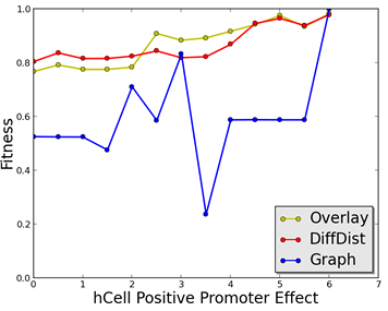
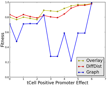
Figure 7.1: Fitness function evaluation on polar model with two gene regulatory regions removed independently and gradually returned. The x-axis shows the effect value of the knocked out regulatory region. The y-axis presents the tness value assigned to the simulated model with a given promoter e ect. The graph edit distance function tness is shown in yellow, overlay in blue, and difference distributions in red.

Figure 7.2: A cellular morphology generated in CellSim using a model with small head and tail regulatory region e ects as well as its graph representation.

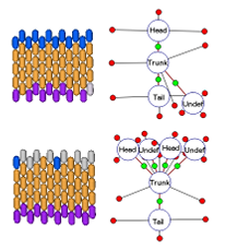
when it is compared against the target graph, lowering the tness value signi cantly. In the case with the worm in Figure 7.2, it got assigned a graph edit distance of 6000 and the tness value of 0.45.

In addition to evaluating the tness functions on independent hCell and tCell knockouts, the evaluators were tested on a combined knockout performed on the polar model, where both hCell and tCell regulatory regions were knocked out simultaneously. Figure 7.3 plots the tness landscapes of a model where both hCell and tCell promoter genes are knocked out at the start and gradually restored to the model. In the gure, the x-axis shows the regulatory region e ect of hCell, the y-axis the e ect of tCell, and the z-axis the tness value assigned by a given tness function to the simulation outcome.

The overlay (Fig. 7.3(a)) and the di erence distributions (Fig. 7.3(b)) fitness functions performed well in this evaluation, yielding gradual and therefore searchable fitness landscapes. The graph edit distance fitness function (Fig. 7.3(c)) produced a

(a) Overlay fitness function performance.

(b) Difference distributions fitness function performance.

(c) Graph edit distance fitness function performance.

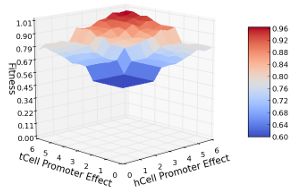
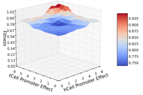
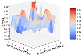
Figure 7.3: Fitness function evaluation of the polar model with hCell and tCell promoters knocked out and gradually returned. very rough surface with many local maxima.

An interesting feature of the resultant graphs for the overlay and difference distributions fitness landscapes was the at rectangular area in the x-axis range [0, 2.27] and the y-axis range [0,2.27] where the tness did not change a lot despite the promoter effect increase. The simulation outcomes with regulatory region promoter effects
within that range did not contain any hCell and tCell molecules. I hypothesized that due to relatively high decay rates (0.2) of the hCell and tCell molecules in the polar regeneration model, the injected hCell and tCell were not able to stabilize with small promoter region effects for these resources. Only at effects of about 2.27 the regulatory region e ects were able to overcome the decay rate and stabilize the examined resources at concentrations higher than zero.

To test the hypothesis that decay rates were a ecting the tness landscapes, the decay rates of hCell and tCell in the polar model were lowered from 0.2 to 0.075. Decay rates lower than 0.075 cause the stable concentrations of hCell and tCell to become very large, and therefore were not considered. Using the models with lower decay rates, the tness values assigned to the simulated models were plotted with gradually increasing regulatory region effects (Fig. 7.4). The resultant overlay and difference distributions fitness landscapes plots show that the lower decay rates allowed the hCell and tCell molecules to start producing at lower fitness values, causing the at areas of the landscape to become smaller (Fig. 7.4(a) and 7.4(b)). The lower decay rate also greatly increased the areas with high fitness values in overlay and graph edit distance fitness landscapes, making those landscapes highly
searchable. It it curious to note that while the graph edit distance and overlay maximum

(b) Difference distributions tness function performance.

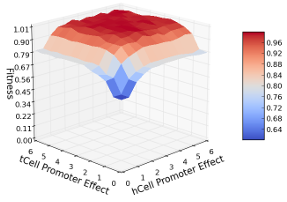
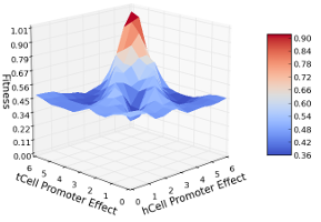
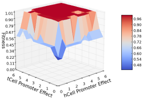
Figure 7.4: Fitness function evaluation of the polar model with low hCell and tCell decay rates in which hCell and tCell regulatory regions were knocked out and gradually returned.

and minimum fitness values stayed in the same range as in the experiment with higher hCell and tCell decay rates, the lowest fitness value of di erence distributions dropped from 0.76 to 0.53. Comparing the difference distributions fitness landscapes of the two experiments (Fig. 7.3(b) and 7.4(b)), it can be seen that the landscape in Figure 7.4(b) is a lot steeper and spans a larger part of the z-axis space, ranging from 0.53 to 1.0. This can be explained by the higher stable hCell and tCell concentrations in the model with lower decay rates. Since the difference distributions evaluator relies on the differences in molecular concentration, models with knocked out regions differ more from the target with high stable concentrations compared to the target with lower stable concentrations.

To conduct a more formal evaluation of the fitness landscapes in Figures 7.3 and 7.4, the landscapes were compared to the landscape of an ideal fitness function. Also the at regions in the resultant fitness landscapes were analyzed and the local maxima were counted. For simplicity, an ideal fitness function landscape is a plane that intersects the points at the minimum and the maximum region promoter effects (that is, a plane that intersects (0,0) and (6,6) where the fitness values for models with hCell and tCell regulatory region effects are 0 and 1 respectively). For each point in the fitness landscape, the expected ideal fitness function point was computed, and the sum squared difference between the ideal and the actual fitness values were calculated. The total sum of all the differences between ideal and actual fitness values yielded the value we used to rank fitness functions. Table 7.3 ranks the tness landscapes from Figures 7.3 and 7.4 by their difference from the ideal fitness function landscape. The smaller values in the table indicate that the fitness landscapes are more similar to the ideal, while larger values show that the fitness landscape differs from that of the ideal landscape.

Table 7.3: Comparison of fitness function landscapes to the ideal fitness function landscape.

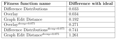
The difference distributions and overlay fitness functions are ranked first, since they show the smoothest transition in the landscape. Prior to evaluation, the graph edit distance fitness function landscapes were expected to perform the worst for models with both normal and low decay rates. However, the graph edit distance landscape for a model with the normal decay rate turned out to be more similar to the ideal fitness function than the overlay and difference distribution landscapes for models with low decay rates. Each fitness landscape was evaluated by examining its at areas and local maxima. The a fitness of a landscape was analyzed by calculating the number of at surfaces, where a at surface consists of at least three adjacent points with the same fitness value. Also the analysis of how much of the total landscape surface is occupied by at areas was performed. Specifically, the percentage occupied by the biggest at surface and the sum of all at surfaces were calculated. Table 7.4 presents the data obtained during the landscape a fitness analysis calculated for the three fitness functions, sorted by the total at area percentage.

Table 7.4: Statistics obtained from analyzing the a fitness of the fitness landscapes. The first column shows the name of the landscape analyzed. Di Dist refers to the difference distributions evaluator and Graph to the graph edit distance evaluator. The second column presents the total number of at surfaces in the landscape, the third column shows the percentage of the total landscape occupied by the biggest at surface, and the last column shows the percentage of the landscape occupied by the flat surfaces.

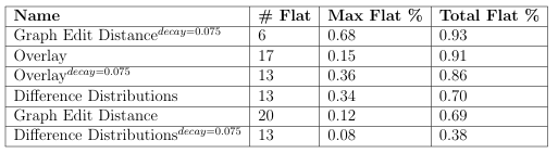
As expected from the landscape figures, the graph edit distance landscape for the model with low decay rate has the largest percentage occupied by the at areas. The landscape also yielded the biggest at surface and the smallest number of at areas. In Figure 7.4(c), the largest at area is the surface marked dark red, where the individual fitnesses are 1.0. The difference distributions fitness function for a model with low decay rate yielded a landscape with the smallest percentage occupied by at areas. Due to fluctuations in molecular concentrations and the difference distributions high reliance on the metabolic state of the worm, fitness values fluctuated as well, thus producing a rougher landscape. It is interesting to note that the landscape that generated the majority of at areas was formed by the graph edit distance fitness function. In Figure 7.3(c), the landscape is very rough, with lots of jumps throughout, but most of the jumps form small at surfaces of at least three points, which are deemed as at surfaces by the analysis. To analyze the roughness of the fitness landscapes, the number of local maxima found in a landscape was counted. Here, local maximum is one or more points with very similar tness values surrounded by points with smaller fitness (z-axis) values (Fig. 7.5). As expected, the graph edit distance tness landscape proved to be the roughest, having the largest number of local maxima. Due to the lack of at areas in
the difference distributions fitness landscapes as well as the fitness fluctuations that tend to happen in this fitness function, the difference distributions fitness landscapes proved to be next in landscape roughness. The overlay fitness landscapes proved to be very smooth in the roughness evaluation with a very small number of local maxima present.

Table 7.5: Statistics obtained from analyzing the roughness of the fitness landscapes. The first column shows the name of the fitness landscape, and the second column shows the number of local maxima in the landscape.

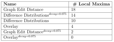
To further test the utility of the proposed fitness functions, an evolutionary search for the target model was set up, where the starting model of normal decay rate had the genes promoting head and tail regions knocked out. As the search progressed, at the end of each generation a mutation operator modified the regulatory region
effects, a 2-point crossover was performed on the selected individuals, and the model was simulated in the cellular platform for 200 steps until the metabolic stability was achieved. At step 200, a transverse cut was performed on the worm and the simulation was ran for 200 more steps to allow the regeneration processes to take place. Once the simulation was finished, simulation outcomes were evaluated against the target outcome using one of the fitness evaluators. To evaluate the performance of different evaluators on the evolutionary search, a time series graph for each of the three fitness functions was created (Fig.7.5). In a time series graph, the highest fitness value found in a given generation (y-axis) is plotted against time, or the generation count (x-axis).

Figure 7.5: A time series graph for an evolutionary search for a target capable of producing stable head and tail regions.

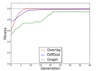
Figure 7.5 presents the average time series for five consecutive GA searches. In each of the five searches, the overlay and difference distributions fitness functions were able to find the target relatively fast: overlay in 10 and difference distributions in 17 generations. The graph edit distance fitness function found the target in four of the
five of the GA search runs; however, it got stuck on the local maximum during the fifth run, where the fitness did not go over 0.71 even after the evolutionary search ran for 500 generations. This explains why the graph edit distance time series curve in Figure 7.5 is significantly below the overlay and graph edit distance curves. The
possibility of the search getting stuck at a local maximum can be visually explained by the examination of the fitness landscape for the graph edit distance (Fig. 7.3(c)).

Due to a large number of local maxima, it is very easy for the search to get stuck in one of them.

7.2.1 Difference Distributions Fitness Function Evaluation

In order to construct a histogram in the difference distributions evaluator, each cell in the cellular morphology has to be compared against every other cell, making the complexity of the algorithm O(N2). Considering that the creation of difference distributions has to be performed for every model generated during the evolutionary search process, it is crucial to construct distributions quickly and efficiently. Speedup and efficiency are the main reasons for rewriting the Python module for creating difference distribution histograms into a C implementation.
To access the speedup provided by the C implementation of difference distribution histogram creator, histograms were constructed for several CellSim simulation snap shots. The runtime of histogram construction for C and Python implementations as well as the speedup achieved by the new C implementation are shown in Table 7.6.
The conversion of the difference distributions histogram creator code from Python to C has provided a 72 times speedup on average as seen in Table 7.6. This distinction is crucial, especially in such a time-dependent application as the CellSim genetic algorithm, which has to process hundreds of morphologies in order to nd the target. In addition to providing the speedup assessment of the histogram creator C implementation, this work examined how intuitive the difference distributions evaluator is at assigning fitness values to various morphologies. The difference distributions fitness function was used to evaluate the polar regeneration model from Section 1.4.3

Table 7.6: The runtime of di erence distribution histogram creator implementations in C and Python for morphology in column one are shown in columns two and three, respectively. The speedup provided by the C implementation of the histogram creator is shown in column four. The last row of the table shows the average runtimes.

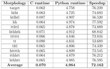
with various permutations of head, trunk, and tail region promoters knocked out. Table 7.7 shows the difference distribution histograms and fitness values assigned by the difference distributions evaluator to the examined models. In the evaluation, the difference samples were collected by using a subunit-to-subunit di erence processor described in Section 4.1, which were in turn converted into a ten-bin distribution histogram.
In Table 7.7, the Distribution column shows the distributions created for the evaluated morphologies. In the plot, the x-axis represents bin indexes ranging from 0 to 9, while the y-axis shows the normalized count of samples that fell within a given bin index during the histogram creation.

By examining the distribution plots, it can be seen that the difference distribution histograms for models with knocked out head and tail promoters look very similar.

Variations in the regenerated head and tail thickness on the cut borders are due to the differences in histograms, and thus in fitness values. The same observation is true about histograms for individuals with head and trunk, tail and trunk, and just trunk regions knocked out. Consequently, the individuals with similar difference distributions histograms were assigned similar fitness function values. It is curious to note that the fitness of the model with head, trunk, and tail promoters knocked out is higher than the fitness of the models with only trunk and
tail genes knocked out. For the model with three knocked out region promoters, the histogram differences are only attributed to the differences in sub unit locations. There are few differences in molecular concentrations in the model because the con centrations of assessed molecules (head, trunk, and tail region promoters) are all zero. This behavior of the di erence distributions tness function is not very favorable from the evolutionary search perspective, as it favors models that may sway the search and potentially cause it to go in the wrong direction.

Table7.7: Difference distributions formor phologies with different gene knockouts performed.The rstro win the table presents the difference distribution data for the target morphology.

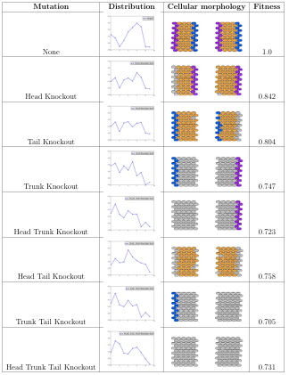
CHAPTER 8

CONCLUSIONS

8.1 Automation of Search for Regeneration Models

This work automated the search for planarian regeneration models that t the experiments reported in the literature. To this end, a flexible evolutionary search, a cellular simulation platform, and a database of planarian experiments have been combined. Several flexible fitness functions have been implemented in order to support the search for different features of planarian regeneration models, such as shape, metabolic networks, and genome.

The automated platform has provided extraction of morphologies and experiments from the Planform database of planarian experiments and reduced the manual design and parameter tuning of models in the CellSim platform. The extracted planarian experiment descriptions can be automatically applied to the cellular morphologies in CellSim by specifying the name of the experiment and the cellular morphology to be manipulated. This work performed the initial assessment of fitness functions that are capable of guiding the evolutionary search most effectively. Evaluation of fitness landscapes produced by the overlay, graph edit distance, and difference distributions fitness functions shows that the graph edit distance evaluator is not as robust as the overlay and difference distribution evaluators due to the roughness of the surface and the potential of getting stuck at local maxima. The overlay and difference distributions fitness functions proved to be robust, and were capable of finding a target individual within 15 generations on a simple evolutionary search run. A closer look at the difference distributions fitness function showed that this evaluator does not always produce fitness values favorable to the evolutionary search. In short, out of the fitness functions examined, the overlay evaluator proved to be the most intuitive from the evolutionary standpoint as well as robust.

All in all, the automated components implemented as a part of this work provided a good start for finding new models of planarian regeneration against the experiments reported in the literature.

8.2 Future Work

8.2.1 Organs

This work used the abstracted representations of planaria worms by considering the region information of the morphologies. To expand the representational complexity of planaria worms, the next step of this research will be to add organ support to the simulation platform and the fitness functions. The organ support to the simulation platform can be added by introducing a combination of indicator molecules representing organs.

8.2.2 Combination of Fitness Functions

The three fitness functions implemented in this work provide different assessments of planaria worm features. As discussed in Section 1.1, the main reasons for having a multi-objective fitness function is to provide multiple possible directions of the evolutionary search and speed up the search. This work evaluated the fitness functions
separately. However, for future work it is crucial to assess fitness function performance when the functions are used in combination with each other. It will be equally important to determine how much each fitness function should contribute to the final fitness used to guide the evolutionary search.

8.2.3 Cellular Morphologies Beyond One Layer

In this work, the morphology abstractions consisted only of a single layer of cells. As a part of future studies, it will be interesting to examine morphologies that not only contain organs but also a more complex shape consisting of several layers of cells.

REFERENCES

[1] K. Agata, T. Tanaka, C. Kobayashi, K. Kato, and Y. Saitoh. Intercalary regeneration in planarians. Developmental Dynamics, 226(2):308316, 2003.

[2] A. Senchez Alvarado, P.W. Reddien, A. Bermange, N. Oviedo, and S.M.C. Robb. Functional studies of regeneration in the planarian schmidtea mediterranea. Developmental Biology, 259:525, 2003.

[3] T. Andersen, R. Newman, and T. Otter. Shape homeostasis in virtual embryos. Arti cial Life, 15(2):161183, 2009.

[4] A.Rosenfeld and J.Pfaltz. Sequential operations in digital picture processing. J. ACM, 13:471494, 1966.

[5] R. A. Baldock, J. B. L. Bard, A. Burger, N. Burton, J. Christiansen, G. Feng, B. Hill, D. Houghton, M. Kaufman, J. Rao, J. Sharpe, A. Ross, P. Stevenson, S. Venkataraman, A. Waterhous, Y. Yang, and D. R. Davidson. Emap and
emage: A framework for understanding spatially organized data. Neuroinfor matics, 1:309325, 2003.

[6] T. Beck, H. Morgan, A. Blake, S. Wells, J. M. Hancock, and A. Mallont. Practical application of ontologies to annotate and analyse large scale raw mouse phenotype data. BMC Bioinformatics, 10, 2009.

[7] K.D. Birnbaum and A. Sanchez Alvarado. Slicing across kingdoms: regeneration in plants and animals. Cell, 132:697710, 2008.

[8] F. Brown and C. Chow. Di erentiation between clockwise and counterclockwise magnetic rotation by the planarian dugesia-dorotocephala. Physiological Zoology, 48:168176, 1975.

[9] F. Brown and Y. Park. Seasonal variations in sign and strength of gamma-taxis in planarians. Nature, 202:469471, 1964.

[10] F. Brown and Y. Park. A persistent monthly variation in responses of planarians to light and its annual modulation. International Journal of Chronobiology, 3:5762, 1975.

[11] H.M. Brown, H. Ito, and T.E. Ogden. Spectral sensitivity of the planarian ocellus. Journal of General Physiology, 51:255260, 1968.

[12] M. Budnikova, J. W. Habig, D. Lobo, N. Cornia, M. Levin, and T. Andersen. De sign of a exible component gathering algorithm for converting cell-based models to graph representations for use in evolutionary search. BMC Bioinformatics 2014, 15, 2014.

[13] Jr. F.A. Brown. E ects and after-e ects on planarians of reversals of the horizontal magnetic vector. Nature, 209:533535, 1966.

[14] D. Fulgheri and P. Messeri. The use of 2 di erent reinforcements in light darkness discrimination in planaria. Bollettino- Societa Italiana Biologia Sperimentale, 49:11411145, 1973.

[15] A. Gierer and H. Meinhardt. A theory of biological pattern formation. Kyber netik, 12(1):3039, 1972.

[16] Richard Hacker. Certi cation of algorithm 112: Position of point relative to polygon. Communications of the ACM, 5:606, 1962.

[17] K. Kato, H. Orii, K. Watanabe, and K. Agata. The role of dorsoventral inter action in the onset of planarian regeneration. Development, 126(5):10311040, 1999.

[18] A. Konaka, D. W. Coitb, and A. E. Smithc. Multi-objective optimization using genetic algorithms: A tutorial. Reliability Engineering and System Safety, 91:9921007, 2006.

[19] C.S. Lange and V.E. Steele. The mechanism of anterior-posterior polarity control in planarians. Di erentiation, 11(1):112, 1978.

[20] Yiu-Wing Leung, Senior Member, and Yuping Wang. Multiobjective programming using uniform design and genetic algorithm. IEEE Trans. Syst. Man Cyber. C, 30:293304, 2000.

[21] M. Levin. The wisdom of the body: future techniques and approaches to morphogenetic elds in regenerative medicine, developmental biology and cancer. Regenerative Medicine, 6:667673, 2011.

[22] M. Levin. Morphogenetic elds in embryogenesis, regeneration, and cancer: non local control of complex patterning. Biosystems, 109:243261, 2012.

[23] D. Lobo, W.S. Beane, and M. Levin. Modeling planarian regeneration: A primer for reverse-engineering the worm. PLoS Comput Biol, 8(4), 2012.

[24] D. Lobo, T. J. Malone, and M. Levin. Towards a bioinformatics of patterning: a computational approach to understanding regulative morphogenesis. Biology Open, 2(2):156169, 2012.

[25] D. Lobo, T. J. Malone, and M. Levin. Planform: an application and database of graph-encoded planarian regenerative experiments. Bioinformatics, 29(8):1098 1100, 2013.

[26] D. Lobo, T. J. Malone, and M. Levin. Towards a bioinformatics of patterning: a computational approach to understanding regulative morphogensis. Biology Open, 2(2):156169, 2013.

[27] A. M. Maglia, J. L. Leopold, L. A. Pugener, and S. Gauch. An anatomical ontology for amphibians. Paci c Symposium on Biocomputing, 12:367378, 2007.

[28] P.R. Mason. Chemo-klino-kinesis in planarian food location. Animal Behaviour, 23:460469, 1975.

[29] H. Meinhardt. Models for the generation and interpretation of gradients. Cold Spring Harbor Perspectives in Biology, 1(4), 2009.

[30] S. Miyamoto and A. Shimozawa. Chemotaxis in the freshwater planarian dugesia japonica-japonica. Zoological Science (Tokyo), 2:389396, 1985.

[31] T.H. Morgan. Experimental studies of the regeneration of planaria maculata. Arch Entwickelingsmech Org, 7:364397, 1898.

[32] M. Neuhaus and H. Bunke. Bridging the Gap Between Graph Edit Distance and Kernel Machines, chapter Chapter 3. Graph Edit Distance. World Scienti c, Singapore, 2007.

[33] P.A. Newmark and A. Sanchez Alvarado. Not your fathers planarian: a classic model enters the era of functional genomics. Nat Rev Genet, 3(3):2109, March 2002.

[34] R. Osada, T. Funkhouser, B. Chazelle, and D. Dobkin. Matching 3d models with shape distributions. International Conference of Shape Modeling and Applications, pages 154166, 2001.

[35] P.S. Pallas. Spicilegia zoologica quibus novae imprimis et obscurae animalium species iconibus, descriptionibus atque commentariis illustrantur. Berolini, Prostant, Apud Gottl., 8(4), 1774.

[36] P.N. Robinson and S. Mundlos. The human phenotype ontology. Clinical Genetics, 77:525534, 2010.

[37] R. Sarker, T. Ray, and O. Grandstrand, editors. Agent Based Evolutionary Search, chapter Agent Based Evolutionary Approach: An Introduction. Springer Verlag, Berlin, Heidelberg, 2010.

[38] J.M.W. Slack. A serial threshold theory of regeneration. Journal of Theoretical Biology, 82(1):105140, 1980.

[39] A.M. Turing. The chemical basis of morphogenesis. Philosophical Transactions of the Royal Society of London. Series B, Biological Sciences, 273(641):3772, 1952.

What's On

Dissertation Example -EVOLUTIONARY SEARCH FOR MODELS OF PLANARIAN REGENERATION USING EXPERIMENTAL DATA

EVOLUTIONARY SEARCH FOR MODELS OF PLANARIAN REGENERATION USING EXPERIMENTAL DATA